Calculating The Gaussian Expected Maximum
In generating a sample of n datapoints drawn from a normal/Gaussian distribution, how big on average the biggest datapoint is will depend on how large n is. I implement a variety of exact & approximate calculations from the literature in R to compare efficiency & accuracy.
In generating a sample of n datapoints drawn from a normal/Gaussian distribution with a particular mean/SD, how big on average the biggest datapoint is will depend on how large n is. Knowing this average is useful in a number of areas like sports or breeding or manufacturing, as it defines how bad/good the worst/best datapoint will be (eg. the score of the winner in a multi-player game).
The order statistic of the mean/average/expectation of the maximum of a draw of n samples from a normal distribution has no exact formula, unfortunately, and is generally not built into any programming language’s libraries.
I implement & compare some of the approaches to estimating this order statistic in the R programming language, for both the maximum and the general order statistic. The overall best approach is to calculate the exact order statistics for the n range of interest using numerical integration via
lmomcoand cache them in a lookup table, rescaling the mean/SD as necessary for arbitrary normal distributions; next best is a polynomial regression approximation; finally, the Elfving correction to the Blom 195868ya approximation is fast, easily implemented, and accurate for reasonably large n such as n > 100.
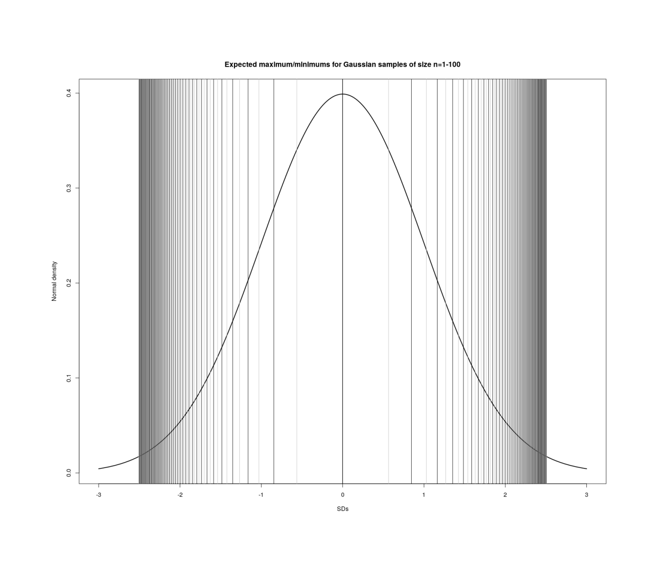
Visualizing maxima/minima in order statistics with increasing n in each sample (1–100).
Approximation
Monte Carlo
Most simply and directly, we can estimate it using a Monte Carlo simulation with hundreds of thousands of iterations:
scores  <- function(n, sd) { rnorm(n, mean=0, sd=sd); }
gain    <- function(n, sd) { scores <- scores(n, sd)
                             return(max(scores)); }
simGain <- function(n, sd=1, iters=500000) {
                             mean(replicate(ie.s, gain(n, sd))); }
But in R this can take seconds for small n and gets worse as n increases into the hundreds as we need to calculate over increasingly large samples of random normals (so one could consider this 𝓞(n)); this makes use of the simulation difficult when nested in higher-level procedures such as anything involving resampling or simulation. In R, calling functions many times is slower than being able to call a function once in a ‘vectorized’ way where all the values can be processed in a single batch. We can try to vectorize this simulation by generating n ⋅ i random normals, group it into a large matrix with n columns (each row being one n-sized batch of samples), then computing the maximum of the i rows, and the mean of the maximums. This is about twice as fast for small n; implementing using rowMaxs from the R package matrixStats, it is anywhere from 25% to 500% faster (at the expense of likely much higher memory usage, as the R interpreter is unlikely to apply any optimizations such as Haskell’s stream fusion):
simGain2 <- function(n, sd=1, iters=500000) {
    mean(apply(matrix(ncol=n, data=rnorm(n*iters, mean=0, sd=sd)), 1, max)) }

library(matrixStats)
simGain3 <- function(n, sd=1, iters=500000) {
    mean(rowMaxs(matrix(ncol=n, data=rnorm(n*iters, mean=0, sd=sd)))) }
Each simulate is too small to be worth parallelizing, but there are so many iterations that they can be split up usefully and run with a fraction in a different process; something like
library(parallel)
library(plyr)
simGainP <- function(n, sd=1, iters=500000, n.parallel=4) {
   mean(unlist(mclapply(1:n.parallel, function(i) {
    mean(replicate(ie.s/n.parallel, gain(n, sd))); })))
}
We can treat the simulation estimates as exact and use memoization such as provided by the R package memoise to cache results & never recompute them, but it will still be slow on the first calculation. So it would be good to have either an exact algorithm or an accurate approximation: for one of analyses, I want accuracy to ±0.0006 SDs, which requires large Monte Carlo samples.
Upper Bounds
The maximum of any distribution remarkably turns out to asymptotically converge to one of three distributions (the Fisher-Tippett-Gnedenko theorem); in this case of normal & exponential variables, the Gumbel distribution.
To summarize the Cross Validated discussion: the simplest upper bound is , which makes the diminishing returns clear. Implementation:
upperBoundMax <- function(n, sd=1) { sd * sqrt(2 * log(n)) }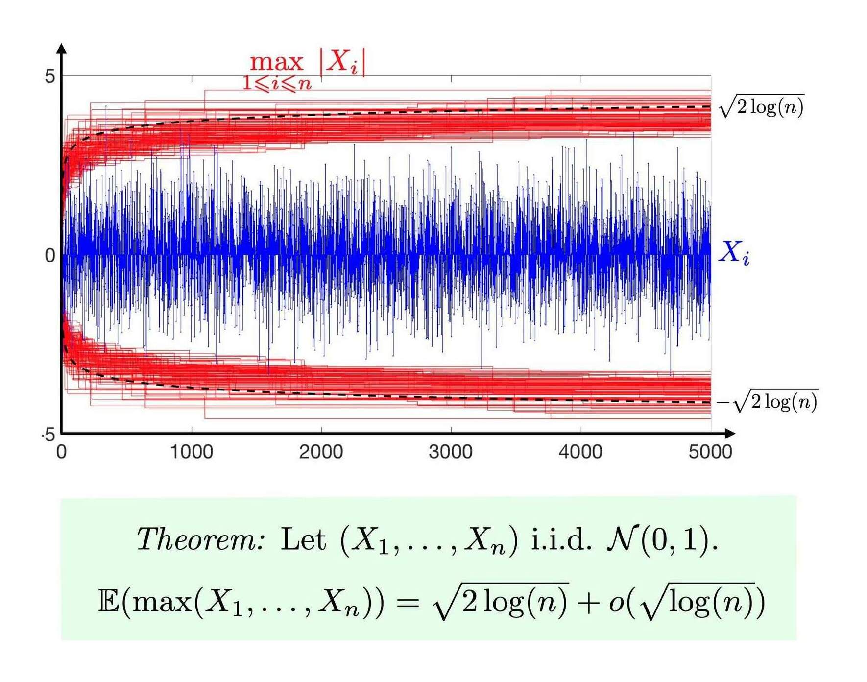
The max central limit theorem visualized (Gabriel Peyré)
Most of the approximations are sufficiently fast as they are effectively 𝓞(1) with small constant factors (if we ignore that functions like Φ−1/qnorm themselves may technically be 𝓞(log(n)) or 𝓞(n) for large n). However, accuracy becomes the problem: this upper bound is hopelessly inaccurate in small samples when we compare to the Monte Carlo simulation. Others (also inaccurate) include and :
upperBoundMax2 <- function(n, sd=1) { ((n-1) / sqrt(2*n - 1)) * sd }
upperBoundMax3 <- function(n, sd=1) { -qnorm(1/(n+1), sd=sd) }
Formulas
Blom 195868ya, Statistical estimates and transformed beta-variables provides a general approximation formula 𝔼(r,n), which specializing to the max (𝔼(n,n)) is ; α = 0.375 and is better than the upper bounds:
blom1958 <- function(n, sd=1) { alpha <- 0.375; qnorm((n-alpha)/(n-2*alpha+1)) * sd }Elfving 1947, apparently, by way of Mathematical Statistics, Wilks 196264ya, demonstrates that Blom 1958’s approximation is imperfect because actually α = π⧸8, so:
elfving1947 <- function(n, sd=1) { alpha <- pi/8; qnorm((n-alpha)/(n-2*alpha+1)) * sd }(Blom 195868ya appears to be more accurate for n < 48 and then Elfving’s correction dominates.)
Harter 1961 elaborated this by giving different values for α, and Royston 1982 provides computer algorithms; I have not attempted to provide an R implementation of these.
probabilityislogic offers a 2015 derivation via the beta-F compound distribution1:
and an approximate (but highly accurate) numerical integration as well:
pil2015 <- function(n, sd=1) { sd * qnorm(n/(n+1)) * { 1 +
    ((n/(n+1)) * (1 - (n/(n+1)))) /
    (2*(n+2) * (pnorm(qnorm(n/(n+1))))^2) }}
pil2015Integrate <- function(n) { mean(qnorm(qbeta(((1:10000) - 0.5) / 10000, n, 1))) + 1}
The integration can be done more directly as
pil2015Integrate2 <- function(n) { integrate(function(v) qnorm(qbeta(v, n, 1)), 0, 1) }Another approximation comes from Chen & Tyler 1999: . Unfortunately, while accurate enough for most purposes, it is still off by as much as 1 IQ point and has an average mean error of −0.32 IQ points compared to the simulation:
chen1999 <- function(n, sd=1){ qnorm(0.5264^(1/n), sd=sd) }

approximationError <- sapply(1:1000, function(n) { (chen1999(n) - simGain(n)) * 15 })
summary(approximationError)
#       Min.    1st Qu.     Median       Mean    3rd Qu.       Max.
# −0.3801803 −0.3263603 −0.3126665 −0.2999775 −0.2923680  0.9445290
plot(1:1000, approximationError,  xlab="Number of samples taking the max", ylab="Error in 15*SD (IQ points)")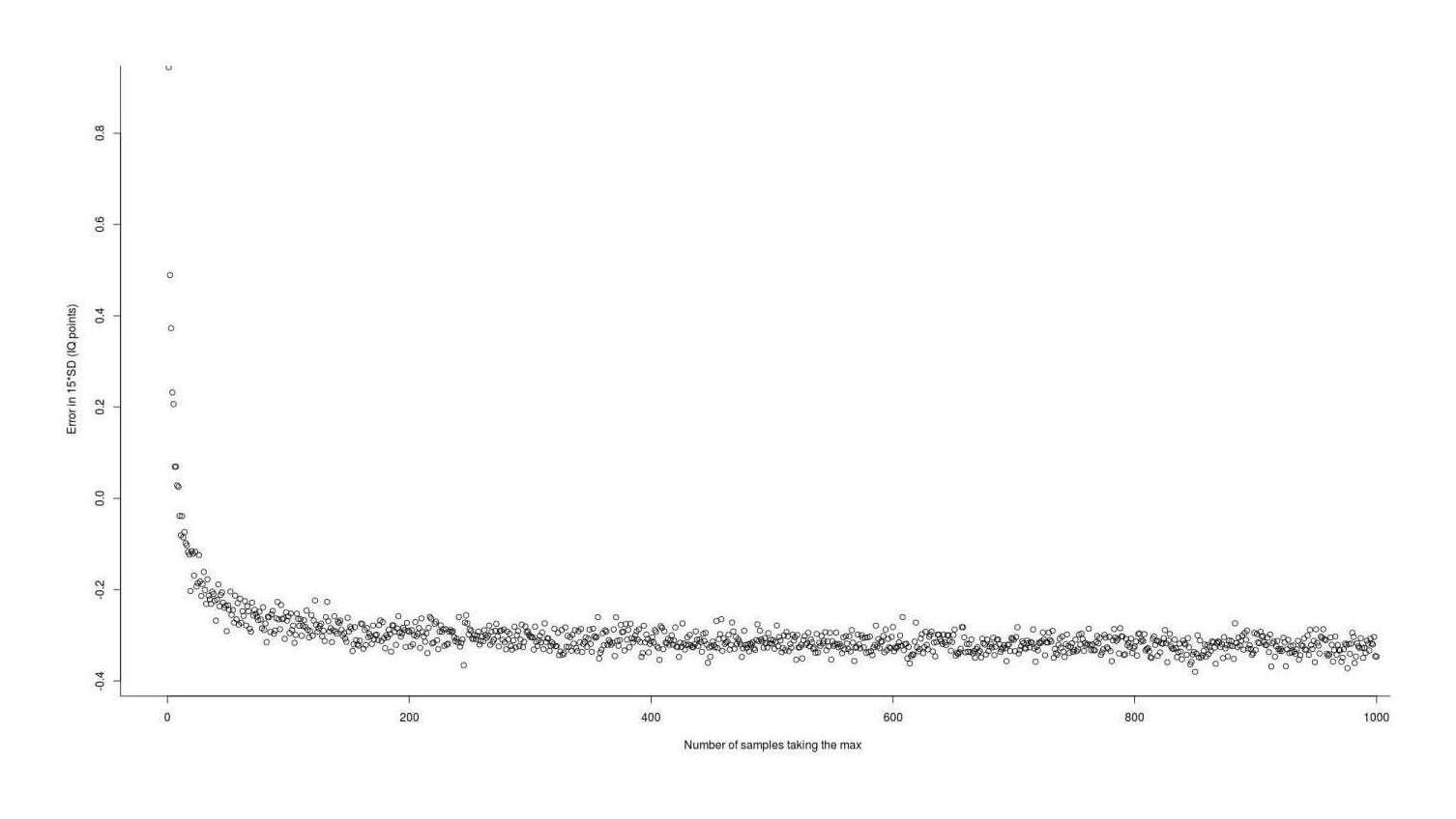
Error in using the Chen & Tyler 199927ya approximation to estimate the expected value (gain) from taking the maximum of n normal samples
Polynomial Regression
From a less mathematical perspective, any regression or machine learning model could be used to try to develop a cheap but highly accurate approximation by simply predicting the extreme from the relevant range of n = 2–300—the goal being less to make good predictions out of sample than to interpolate/memorize as much as possible in-sample.
Plotting the extremes, they form a smooth almost logarithmic curve:
df <- data.frame(N=2:300, Max=sapply(2:300, exactMax))
l <- lm(Max ~ log(N), data=df); summary(l)
# Residuals:
#         Min          1Q      Median          3Q         Max
# −0.36893483 −0.02058671  0.00244294  0.02747659  0.04238113
# Coefficients:
#                Estimate  Std. Error   t value   Pr(>|t|)
# (Intercept) 0.658802439 0.011885532  55.42894 < 2.22e-16
# log(N)      0.395762956 0.002464912 160.55866 < 2.22e-16
#
# Residual standard error: 0.03947098 on 297 degrees of freedom
# Multiple R-squared: 0.9886103,   Adjusted R-squared: 0.9885719
# F-statistic: 25779.08 on 1 and 297 DF,  p-value: < 2.2204e-16
plot(df); lines(predict(l))
This has the merit of simplicity (function(n) {0.658802439 + 0.395762956*log(n)}), but while the R2 is quite high by most standards, the residuals are too large to make a good approximation—the log curve overshoots initially, then undershoots, then overshoots. We can try to find a better log curve by using polynomial or spline regression, which broaden the family of possible curves. A 4th-order polynomial turns out to fit as beautifully as we could wish, R2=0.9999998:
lp <- lm(Max ~ log(N) + I(log(N)^2) + I(log(N)^3) + I(log(N)^4), data=df); summary(lp)
# Residuals:
#           Min            1Q        Median            3Q           Max
# −1.220430e-03 −1.074138e-04 −1.655586e-05  1.125596e-04  9.690842e-04
#
# Coefficients:
#                  Estimate    Std. Error    t value   Pr(>|t|)
# (Intercept)  1.586366e-02  4.550132e-04   34.86418 < 2.22e-16
# log(N)       8.652822e-01  6.627358e-04 1305.62159 < 2.22e-16
# I(log(N)^2) −1.122682e-01  3.256415e-04 −344.76027 < 2.22e-16
# I(log(N)^3)  1.153201e-02  6.540518e-05  176.31640 < 2.22e-16
# I(log(N)^4) −5.302189e-04  4.622731e-06 −114.69820 < 2.22e-16
#
# Residual standard error: 0.0001756982 on 294 degrees of freedom
# Multiple R-squared: 0.9999998,   Adjusted R-squared: 0.9999998
# F-statistic: 3.290056e+08 on 4 and 294 DF,  p-value: < 2.2204e-16

## If we want to call the fitted objects:
linearApprox <- function (n) { predict(l, data.frame(N=n)); }
polynomialApprox <- function (n) { predict(lp, data.frame(N=n)); }
## Or simply code it by hand:
la <- function(n, sd=1) { 0.395762956*log(n) * sd; }
pa <- function(n, sd=1) { N <- log(n);
    (1.586366e-02 + 8.652822e-01*N^1 + -1.122682e-01*N^2 + 1.153201e-02*N^3 + -5.302189e-04*N^4) * sd; }
This has the virtue of speed & simplicity (a few arithmetic operations) and high accuracy, but is not intended to perform well past the largest datapoint of n = 300 (although if one needed to, one could simply generate the additional datapoints, and refit, adding more polynomials if necessary), but turns out to be a good approximation up to n = 800 (after which it consistently overestimates by ~0.01):
heldout <- sapply(301:1000, exactMax)
test <- sapply(301:1000, pa)
mean((heldout - test)^2)
# [1] 3.820988144e-05
plot(301:1000, heldout); lines(test)
So this method, while lacking any kind of mathematical pedigree or derivation, provides the best approximation so far.
Exact
The R package lmomco (Asquith 2011) calculates a wide variety of order statistics using numerical integration & other methods. It is fast, unbiased, and generally correct (for small values of n2)—it is close to the Monte Carlo estimates even for the smallest n where the approximations tend to do badly, so it does what it claims to and provides what we want (a fast exact estimate of the mean gain from selecting the maximum from n samples from a normal distribution). The results can be memoized for a further moderate speedup (eg. calculated over n = 1–1000, 0.45s vs 3.9s for a speedup of ~8.7×):
library(lmomco)
exactMax_unmemoized <- function(n, mean=0, sd=1) {
    expect.max.ostat(n, para=vec2par(c(mean, sd), type="nor"), cdf=cdfnor, pdf=pdfnor) }
## Comparison to MC:
# ...         Min.       1st Qu.        Median          Mean       3rd Qu.          Max.
#    −0.0523499300 −0.0128622900 −0.0003641315 −0.0007935236  0.0108748800  0.0645207000

library(memoise)
exactMax_memoized <- memoise(exactMax_unmemoized)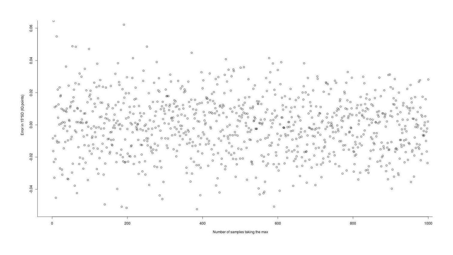
Error in using Asquith 2011’s L-moment Statistics numerical integration package to estimate the expected value (gain) from taking the maximum of n normal samples
Comparison
With lmomco providing exact values, we can visually compare all the presented methods for accuracy; there are considerable differences but the best methods are in close agreement:
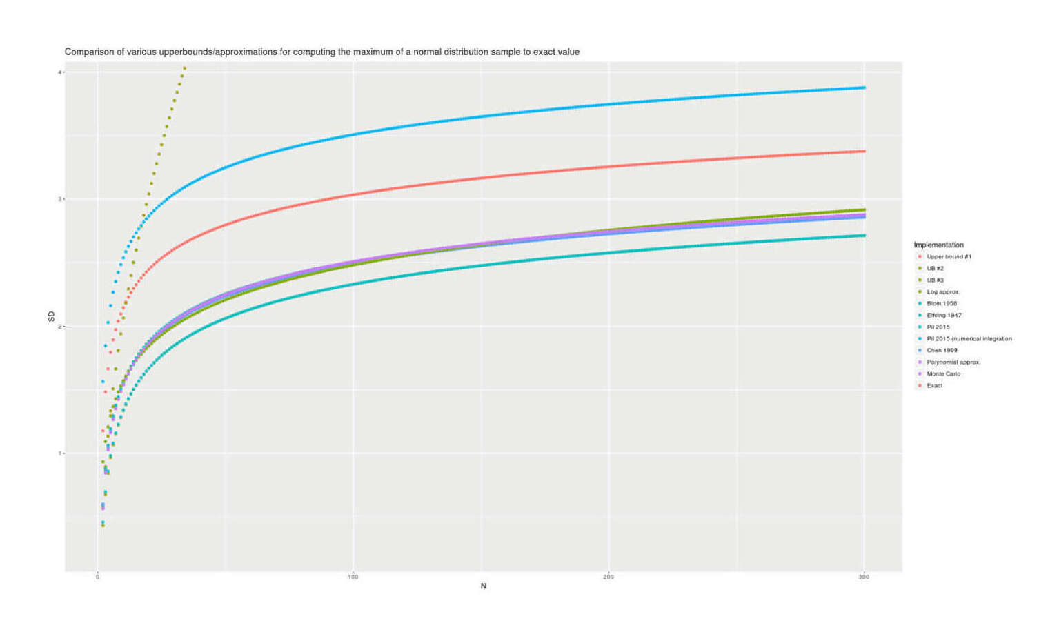
Comparison of estimates of the maximum for n = 2–300 for 12 methods, showing Chen 199927ya/polynomial approximation/Monte Carlo/lmomco are the most accurate and Blom 195868ya/upper bounds highly-inaccurate.
library(parallel)
library(plyr)
scores  <- function(n, sd) { rnorm(n, mean=0, sd=sd); }
gain    <- function(n, sd) { scores <- scores(n, sd)
                             return(max(scores)); }
simGainP <- function(n, sd=1, iters=500000, n.parallel=4) {
   mean(unlist(mclapply(1:n.parallel, function(i) {
    mean(replicate(ie.s/n.parallel, gain(n, sd))); })))
}
upperBoundMax <- function(n, sd=1) { sd * sqrt(2 * log(n)) }
upperBoundMax2 <- function(n, sd=1) { ((n-1) / sqrt(2*n - 1)) * sd }
upperBoundMax3 <- function(n, sd=1) { -qnorm(1/(n+1), sd=sd) }
blom1958 <- function(n, sd=1) { alpha <- 0.375; qnorm((n-alpha)/(n-2*alpha+1)) * sd }
elfving1947 <- function(n, sd=1) { alpha <- pi/8; qnorm((n-alpha)/(n-2*alpha+1)) * sd }
pil2015 <- function(n, sd=1) { sd * qnorm(n/(n+1)) * { 1 +
    ((n/(n+1)) * (1 - (n/(n+1)))) /
    (2*(n+2) * (pnorm(qnorm(n/(n+1))))^2) }}
pil2015Integrate <- function(n) { mean(qnorm(qbeta(((1:10000) - 0.5) / 10000, n, 1))) + 1}
chen1999 <- function(n,sd=1){ qnorm(0.5264^(1/n), sd=sd) }
library(lmomco)
exactMax_unmemoized <- function(n, mean=0, sd=1) {
    expect.max.ostat(n, para=vec2par(c(mean, sd), type="nor"), cdf=cdfnor, pdf=pdfnor) }
library(memoise)
exactMax_memoized <- memoise(exactMax_unmemoized)
la <- function(n, sd=1) { 0.395762956*log(n) * sd; }
pa <- function(n, sd=1) { N <- log(n);
    (1.586366e-02 + 8.652822e-01*N^1 + -1.122682e-01*N^2 + 1.153201e-02*N^3 + -5.302189e-04*N^4) * sd; }

implementations <- c(simGainP,upperBoundMax,upperBoundMax2,upperBoundMax3,blom1958,elfving1947,
    pil2015,pil2015Integrate,chen1999,exactMax_unmemoized,la,pa)
implementationNames <- c("Monte Carlo"",Upper bound #1"",UB #2"",UB #3"",Blom 1958"",Elfving 1947",
    "Pil 2015"",Pil 2015 (numerical integration)"",Chen 1999"",Exact"",Log approx."",Polynomial approx.")
maxN <- 300
results <- data.frame(N=integer(), SD=numeric(), Implementation=character())
for (i in 1:length(implementations)) {
    SD <- unlist(Map(function(n) { implementations[i][[1]](n); }, 2:maxN))
    name <- implementationNames[i]
    results <- rbind(results, (data.frame(N=2:maxN, SD=SD, Implementation=name)))
    }
results$Implementation <- ordered(results$Implementation,
    levels=c("Upper bound #1"",UB #2"",UB #3"",Log approx."",Blom 1958"",Elfving 1947"",Pil 2015",
             "Pil 2015 (numerical integration)"",Chen 1999"",Polynomial approx.", "Monte Carlo", "Exact"))
library(ggplot2)
qplot(N, SD, color=Implementation, data=results) + coord_cartesian(ylim = c(0.25,3.9))

qplot(N, SD, color=Implementation, data=results) + geom_smooth()
And micro-benchmarking them quickly (excluding Monte Carlo) to get an idea of time consumption shows the expected results (aside from Pil 2015’s numerical integration taking longer than expected, suggesting either memoising or changing the fineness):
library(microbenchmark)
f <- function() { sample(2:1000, 1); }
microbenchmark(times=10000, upperBoundMax(f()),upperBoundMax2(f()),upperBoundMax3(f()),
    blom1958(f()),elfving1947(f()),pil2015(f()),pil2015Integrate(f()),chen1999(f()),
    exactMax_memoized(f()),la(f()),pa(f()))
# Unit: microseconds
#                    expr       min         lq          mean     median         uq       max neval
#                     f()     2.437     2.9610     4.8928136     3.2530     3.8310  1324.276 10000
#      upperBoundMax(f())     3.029     4.0020     6.6270124     4.9920     6.3595  1218.010 10000
#     upperBoundMax2(f())     2.886     3.8970     6.5326593     4.7235     5.8420  1029.148 10000
#     upperBoundMax3(f())     3.678     4.8290     7.4714030     5.8660     7.2945   892.594 10000
#           blom1958(f())     3.734     4.7325     7.3521356     5.6200     7.0590  1050.915 10000
#        elfving1947(f())     3.757     4.8330     7.7927493     5.7850     7.2800  1045.616 10000
#            pil2015(f())     5.518     6.9330    10.8501286     9.2065    11.5280   867.332 10000
#   pil2015Integrate(f()) 14088.659 20499.6835 21516.4141399 21032.5725 22151.4150 53977.498 10000
#           chen1999(f())     3.788     4.9260     7.7456654     6.0370     7.5600  1415.992 10000
#  exactMax_memoized(f())   106.222   126.1050   211.4051056   162.7605   221.2050  4009.048 10000
#                 la(f())     2.882     3.8000     5.7257008     4.4980     5.6845  1287.379 10000
#                 pa(f())     3.397     4.4860     7.0406035     5.4785     6.9090  1818.558 10000
Rescaling for Generality
The memoized function has 3 arguments, so memoising on the fly would seem to be the best one could do, since one cannot precompute all possible combinations of the n/mean/SD. But actually, we only need to compute the results for each n.
We can default to assuming the standard normal distribution (𝒩(0,1)) without loss of generality because it’s easy to rescale any normal to another normal: to scale to a different mean μ, one simply adds μ to the expected extreme, so one can assume μ = 0; and to scale to a different standard deviation, we simply multiply appropriately. So if we wanted the extreme for n = 5 for 𝒩(10,2), we can calculate it simply by taking the estimate for n = 5 for 𝒩(0,1) and multiplying by 2⁄1 = 2 and then adding 10 − 0 = 10:
(exactMax(5, mean=0, sd=1)*2 + 10) ; exactMax(5, mean=10, sd=2)
# [1] 12.32592895
# [1] 12.32592895
So in other words, it is unnecessary to memoize all possible combinations of n, mean, and SD—in reality, we only need to compute each n and then rescale it as necessary for each caller. And in practice, we only care about n = 2–200, which is few enough that we can define a lookup table using the lmomco results and use that instead (with a fallback to lmomco for n > 200, and a fallback to Chen et al 199927ya for n > 200026ya to work around lmomco’s bug with large n):
exactMax <- function (n, mean=0, sd=1) {
if (n>2000) {
    chen1999 <- function(n,mean=0,sd=1){ mean + qnorm(0.5264^(1/n), sd=sd) }
    chen1999(n,mean=mean,sd=sd) } else {
    if(n>200) { library(lmomco)
        exactMax_unmemoized <- function(n, mean=0, sd=1) {
            expect.max.ostat(n, para=vec2par(c(mean, sd), type="nor"), cdf=cdfnor, pdf=pdfnor) }
        exactMax_unmemoized(n,mean=mean,sd=sd) } else {

 lookup <- c(0,0,0.5641895835,0.8462843753,1.0293753730,1.1629644736,1.2672063606,1.3521783756,1.4236003060,
  1.4850131622,1.5387527308,1.5864363519,1.6292276399,1.6679901770,1.7033815541,1.7359134449,1.7659913931,
  1.7939419809,1.8200318790,1.8444815116,1.8674750598,1.8891679149,1.9096923217,1.9291617116,1.9476740742,
  1.9653146098,1.9821578398,1.9982693020,2.0137069241,2.0285221460,2.0427608442,2.0564640976,2.0696688279,
  2.0824083360,2.0947127558,2.1066094396,2.1181232867,2.1292770254,2.1400914552,2.1505856577,2.1607771781,
  2.1706821847,2.1803156075,2.1896912604,2.1988219487,2.2077195639,2.2163951679,2.2248590675,2.2331208808,
  2.2411895970,2.2490736293,2.2567808626,2.2643186963,2.2716940833,2.2789135645,2.2859833005,2.2929091006,
  2.2996964480,2.3063505243,2.3128762306,2.3192782072,2.3255608518,2.3317283357,2.3377846191,2.3437334651,
  2.3495784520,2.3553229856,2.3609703096,2.3665235160,2.3719855541,2.3773592389,2.3826472594,2.3878521858,
  2.3929764763,2.3980224835,2.4029924601,2.4078885649,2.4127128675,2.4174673530,2.4221539270,2.4267744193,
  2.4313305880,2.4358241231,2.4402566500,2.4446297329,2.4489448774,2.4532035335,2.4574070986,2.4615569196,
  2.4656542955,2.4697004768,2.4736966781,2.4776440650,2.4815437655,2.4853968699,2.4892044318,2.4929674704,
  2.4966869713,2.5003638885,2.5039991455,2.5075936364,2.5111482275,2.5146637581,2.5181410417,2.5215808672,
  2.5249839996,2.5283511812,2.5316831323,2.5349805521,2.5382441196,2.5414744943,2.5446723168,2.5478382097,
  2.5509727783,2.5540766110,2.5571502801,2.5601943423,2.5632093392,2.5661957981,2.5691542321,2.5720851410,
  2.5749890115,2.5778663175,2.5807175211,2.5835430725,2.5863434103,2.5891189625,2.5918701463,2.5945973686,
  2.5973010263,2.5999815069,2.6026391883,2.6052744395,2.6078876209,2.6104790841,2.6130491728,2.6155982225,
  2.6181265612,2.6206345093,2.6231223799,2.6255904791,2.6280391062,2.6304685538,2.6328791081,2.6352710490,
  2.6376446504,2.6400001801,2.6423379005,2.6446580681,2.6469609341,2.6492467445,2.6515157401,2.6537681566,
  2.6560042252,2.6582241720,2.6604282187,2.6626165826,2.6647894763,2.6669471086,2.6690896839,2.6712174028,
  2.6733304616,2.6754290533,2.6775133667,2.6795835873,2.6816398969,2.6836824739,2.6857114935,2.6877271274,
  2.6897295441,2.6917189092,2.6936953850,2.6956591311,2.6976103040,2.6995490574,2.7014755424,2.7033899072,
  2.7052922974,2.7071828562,2.7090617242,2.7109290393,2.7127849375,2.7146295520,2.7164630139,2.7182854522,
  2.7200969934,2.7218977622,2.7236878809,2.7254674700,2.7272366478,2.7289955308,2.7307442335,2.7324828686,
  2.7342115470,2.7359303775,2.7376394676,2.7393389228,2.7410288469,2.7427093423,2.7443805094,2.7460424475)

 return(mean + sd*lookup[n+1]) }}}
This gives us exact computation at 𝓞(1) (with an amortized 𝓞(1) when n > 200) with an extremely small constant factor (a conditional, vector index, multiplication, and addition, which is overall ~10× faster than a memoized lookup), giving us all our desiderata simultaneously & resolving the problem.
General Order Statistics for the Normal Distribution
One might also be interested in computing the general order statistic.
Some available implementations in R:
numerical integration:
lmomco, withjofn(warning: remember lmomco’s bug with n > 200026ya):j = 9; n = 10 expect.max.ostat(n, j=j, para=vec2par(c(0, 1), type="nor"), cdf=cdfnor, pdf=pdfnor) # [1] 1.001357045evNormOrdStatsinEnvStats(version ≥2.3.0), using Royston 198244ya:library(EnvStats) evNormOrdStatsScalar(10^10,10^10) # [1] 6.446676405 ## Warning message: In evNormOrdStatsScalar(10^10, 10^10) : ## The 'Royston' method has not been validated for sample sizes greater than 2000 using ## the default value of inc = 0.025. You may want to make the value of 'inc' less than 0.025. evNormOrdStatsScalar(10^10,10^10, inc=0.000001) # [1] 6.446676817
Monte Carlo: the simple approach of averaging over i iterations of generating n random normal deviates, sorting, and selecting the
jth order statistic does not scale well due to being 𝓞(n) in both time & space for generation & 𝓞(n ⋅ log(n)) for a comparison sort or another 𝓞(n) if one is more careful to use a lazy sort or selection algorithm, and coding up an online selection algorithm is not a one-liner. Better solutions typically use a beta transformation to efficiently generate a single sample from the expected order statistic:order_rnorminorderstats, withkofn:library(orderstats) mean(replicate(100000, order_rnorm(k=10^10, n=10^10))) # [1] 6.446370373orderinevd, withjofn:library(evd) mean(rorder(100000, distn="norm", j=10^10, mlen=10^10, largest=FALSE)) # [1] 6.447222051
Blom & other approximations:
evNormOrdStatsinEnvStats’s provides as an option the Blom approximation:3When
method="blom", the following approximation to 𝔼(r,n), proposed by Blom (195868ya, pp. 68–75), is used:By default, alpha = 3⁄8 = 0.375. This approximation is quite accurate. For example, for n > 2, the approximation is accurate to the first decimal place, and for n > 9 it is accurate to the second decimal place.
Blom’s approximation is also quoted as:
Elfving’s correction to Blom is the same, yielding:
elfving1947E <- function(r,n) { alpha=pi/8; qnorm((r - alpha) / (n - 2*alpha + 1)) }
elfving1947E(10^10, 10^10)
# [1] 6.437496713
See Also
Appendix
Probability of Bivariate Maximum
Given a sample of n pairs of 2 normal variables A & B which are correlated r, what is the probability Pmax that the maximum on the first variable A is also the maximum on the second variable B? This is analogous to many testing or screening situations, such as employee hiring (“what is the probability the top-scoring applicant on the first exam is the top-scorer on the second as well?”) or athletic contests (“what is the probability the current world champ will win the next championship?”).
Order statistics has long proven that asymptotically, Pmax approaches 1⧸n. Exact answers are hard to find, but confirm the asymptotics; the closest that exists is for an approximation & special-case of the Ali-Mikhail-Haq copula: which roughly indicates that r functions as a constant factor boost in Pmax, and the boost from r fades out as n increases.
As long as r ≠ 1, “the tails will come apart”. n increases the difficult too fast for any fixed r to overcome. This has implications for interpreting extremes and test metrics.
Few are the best at everything.—“the tails come apart” when we look at extremes of multiple traits: the best on one dimension is rarely the best on the second dimension, even if there is a close causal relationship—the tallest basketball player is not the best basketball player, the smartest scientist is not the most influential scientist, the calmest investor is not the richest investor, and so on. This observation can be misinterpreted, and is not necessarily that important: height is certainly useful for basketball players, and the smarter you are, the better your chance of being a great scientist. If we look at the best, they will indeed be well above average on relevant traits, even if they are not the most extreme outlier on all (or any) traits.
How much does best-at-X help Y? But this does raise the question of what the relationship is between the two possible maxima. In other order statistics, an initially small tail effect can become large; a familiar example of a tail effect is the probability of a random sample crossing a threshold, when drawing from populations with different means or standard deviations—the higher the threshold, the bigger the multiplicative increase, and with a not-too-high threshold and a quite small difference in means, one population could completely (and counterintuitively) dominant the sample. Does that happen with the bivariate maximum? More generally, does a given r > 0 increase the probability, how much, and does this probability increase or decrease relative to the 1⧸n baseline?
Let’s consider some cases of r and n:
If r = 1, then Pmax must also always be 1, as the two variables are identical.
For any r, selecting the maximum out of n = 1 is trivial and we can guarantee a Pmax = 1 chance of selecting the maximum
For n = 2, getting the maximum twice out of 2 is easy (we must start at ≥0.5 and go up from there, to 1⁄2 + 1⧸π arcsin(r), so eg. 2⁄3 for r = 0.5).
For larger n, we can simulate out Pmax and see that despite the benefits to increasing averages & reduced regret (eg. for embryo selection), getting the max twice becomes increasingly difficult and out of eg. n = 1 million, becomes near-impossible—even with high r, like r = 0.95 (comparable to test-retest reliability for the SAT).
Eventually, ‘the tails come apart’. Asymptotically, as n increases, the two distributions become independent (Sibuya 1960) and so the probability of the max in one being max in the other approaches 1⧸n. (Srivastava 1967/Mardia 1964 prove this is true of the other extremes as well.) The benefits of an r, however large initially, are not large enough to keep up with the increasing n, and is overwhelmed.
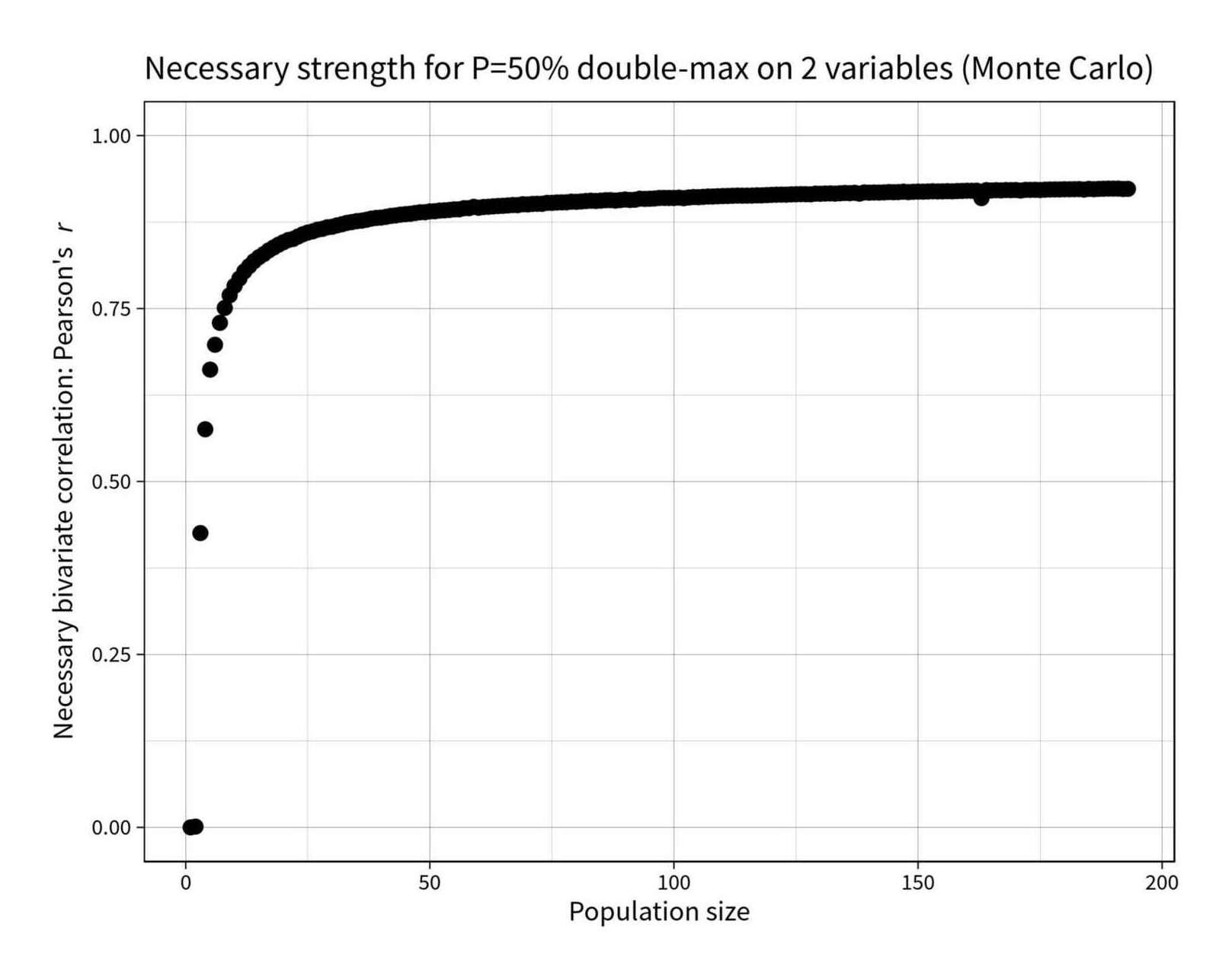
What strength correlation is required in a bivariate sample of n in order to have a 50% chance of the same point being the sample-maximum on both?
find_r_for_topp <- function(n, topp_target=0.5) {
  r_solver <- function(r) {
     topp <- p_max_bivariate_montecarlo(n, r)
     return(abs(topp_target - topp))
   }
  optim(0.94, r_solver, method="Brent", lower=0, upper=1)$par
  }

library(parallel); library(plyr)
rs <- c(0, ldply(mclapply(2:193, find_r_for_topp))$V1)
round(digits=3, rs)
#   [1] 0.000 0.001 0.425 0.575 0.662 0.698 0.729 0.751 0.769 0.783 0.793 0.804 0.811 0.818 0.824 0.829 0.834 0.838 0.842 0.846 0.849 0.851 0.854 0.857 0.860 0.862
#  [27] 0.864 0.865 0.867 0.868 0.870 0.872 0.874 0.875 0.876 0.877 0.878 0.880 0.881 0.881 0.882 0.884 0.885 0.886 0.886 0.887 0.888 0.889 0.889 0.890 0.891 0.892
#  [53] 0.892 0.893 0.893 0.893 0.895 0.895 0.897 0.896 0.897 0.897 0.898 0.898 0.898 0.899 0.900 0.899 0.901 0.900 0.901 0.901 0.901 0.903 0.903 0.903 0.903 0.904
#  [79] 0.904 0.904 0.905 0.905 0.906 0.905 0.906 0.907 0.907 0.906 0.907 0.908 0.907 0.907 0.909 0.908 0.909 0.909 0.910 0.910 0.910 0.910 0.910 0.910 0.910 0.911
# [105] 0.911 0.911 0.912 0.912 0.912 0.913 0.913 0.913 0.913 0.913 0.913 0.913 0.914 0.914 0.914 0.914 0.915 0.915 0.915 0.915 0.915 0.915 0.915 0.915 0.916 0.916
# [131] 0.916 0.916 0.916 0.917 0.917 0.917 0.917 0.916 0.918 0.917 0.918 0.918 0.918 0.918 0.918 0.918 0.919 0.918 0.919 0.919 0.919 0.919 0.919 0.919 0.919 0.920
# [157] 0.919 0.920 0.920 0.920 0.920 0.920 0.910 0.921 0.921 0.921 0.921 0.921 0.921 0.921 0.921 0.922 0.921 0.922 0.921 0.922 0.922 0.922 0.922 0.922 0.922 0.922
# [183] 0.923 0.922 0.923 0.922 0.923 0.923 0.923 0.923 0.923 0.923 0.923

library(ggplot2)
qplot(1:193, rs) + coord_cartesian(ylim=c(0,1)) + ylab(expression("Necessary bivariate correlation: Pearson's"~italic("r"))) +
    xlab("Population size") + ggtitle("Necessary strength for P=50% double-max on 2 variables (Monte Carlo)") +
    theme_linedraw(base_size = 40, base_family="Source Sans Pro") + geom_point(size=10)
Of course, the mean on the second distribution keeps increasing—it just doesn’t increase as fast as necessary to maintain Pmax.
This has some implications. First, it shows that we shouldn’t take too seriously any argument of the form “the max on A is not the max on B, therefore A doesn’t matter to B”, since we can see that this is consistent with arbitrarily high r (even a r = 0.9999 will eventually give such a datapoint if we make n big enough). Second, it shows that Pmax is not that interesting as a measure, since the asymptotic independence means that we may just be “sampling to a foregone conclusion”; anyone evaluating a selection or ranking procedure which puts stress on a candidate being the max on multiple traits (instead of having a high absolute value on traits) should think carefully about using such an (often unnatural) zero-one loss (Aut Caesar, aut nihil?) & its perverse consequences, like guaranteeing that the best candidate all-around will rarely or never be the maximum on any or all traits.
Ali-Mikhail-Haq Copula
The relationship between r and n can be seen more explicitly in a special case formula for the Ali-Mikhail-Haq copula, which also shows how r fades out with n. Matt F. has provided an analytic expression by using a different distribution, the Ali-Mikhail-Haq (AMH) copula, which approximates the normal distribution for the special-case 0 < r < 0.5, if r is converted to the Ali-Mikhail-Haq’s equivalent Kendall’s tau correlation instead:
First we choose the parameter θ to get Kendall’s tau to agree for the two distributions:
…θ = 3r - 2r2 is a decent approximation to the first equation.
Then we can calculate the probability of X and Y being maximized at the same observation:
In the limiting case where r = 1⁄2, we have θ = 1, and the probability is 2⧸(1 + n)
In the limiting case of high n, the probability tends to and more precisely .
In general, the probability is
where and is the hypergeometric function.
His identity isn’t a simple one in terms of r, but the necessary θ can be found to high accuracy by numerical optimization of the identity, using R’s built-in numerical optimization routine optim. Then the general formula can be estimated as written, with the main difficulty being where to get the hypergeometric function. The resulting algorithm (an approximation of an exact answer to an approximation) can then be compared to a large (i = 1 million) Monte Carlo simulation: it is good for small n but has noticeable error:
r_to_theta <- function (r) {
   identity_solver <- function(theta, r) {
       target = 2/pi * asin(r)
       theta_guess = 1 - ((2 * ((1 - theta)^2 * log(1 - theta) + theta))/(3 * theta^2))
       return(abs(target - theta_guess)) }

    theta_approx <- optim(0, identity_solver, r=r, method="Brent", lower=0, upper=1)
    theta_approx$par
    }

## The hypergeometric function is valid for all reals, but practically speaking,
## GSL's 'hyperg_2F1' code has issues with NaN once r>0.2 (theta ≈ −2.3); Stéphane Laurent
## recommends transforming (https://stats.stackexchange.com/a/33455/16897) for stability:
Gauss2F1 <- function(a,b,c,x){
    ## "gsl: Wrapper for the Gnu Scientific Library"
    ## https://cran.r-project.org/web/packages/gsl/index.html for 'hyperg_2F1'
    library(gsl)
    if(x>=0 & x<1){
        hyperg_2F1(a,b,c,x)
    }else{
            hyperg_2F1(c-a,b,c,1-1/(1-x))/(1-x)^b
        }
}

## Calculate the exact probability of a double max using the AMH approximation:
p_max_bivariate_amh <- function(n,r) {
  ## only valid for the special-case r=0-0.5:
  if (r > 0.5 || r < 0.0) { stop("AMH formula only valid for 0 <= r <= 0.5") }
    else {
        ## Handle special cases:
        if (r == 0.5) { 2 / 1+n } else {
         if (r == 0) { 1 / n } else {

            theta <- r_to_theta(r)
            t <- theta / (theta - 1)

            t * (Gauss2F1(1, n+1, n+2, t) / (n+1)) -
            2 * n * t^2 * (Gauss2F1(1, n+2, n+3, t) / ((n+1)*(n+2))) -
            (2*n*t)/((n+1)^2) +
           (1/n)
           }
       }
   }
}

## Monte Carlo simulate the AMH approximation to check the exact formula:
p_max_bivariate_amh_montecarlo <- function(n,r, iters=1000000) {
    ## "copula: Multivariate Dependence with Copulas"
    ## https://cran.r-project.org/web/packages/copula/index.html for 'rCopula', 'amhCopula'
    library(copula)
    theta <- r_to_theta(r)
    mean(replicate(ie.s, {
        sample <- rCopula(n, amhCopula(theta))
        which.max(sample[,1])==which.max(sample[,2]) }))
    }

## Monte Carlo simulation of double max using the normal distribution:
p_max_bivariate_montecarlo <- function(n,r,iters=1000000) {
    library(MASS) # for 'mvrnorm'
    mean(replicate(ie.s, {
                sample <- mvrnorm(n, mu=c(0,0), Sigma=matrix(c(1, r, r, 1), nrow=2))
                which.max(sample[,1])==which.max(sample[,2])
                })) }

## Compare all 3:
## 1. approximate Monte Carlo answer for the normal
## 2. exact answer to A-M-H approximation
## 3. approximate Monte Carlo answer to A-M-H approximation
r=0.25
round(digits=3, sapply(2:20, function(n) { p_max_bivariate_montecarlo(n, r) }))
# [1] 0.580 0.427 0.345 0.295 0.258 0.230 0.211 0.193 0.179 0.168 0.158 0.150 0.142 0.136 0.130 0.124 0.120 0.115 0.111
round(digits=3, sapply(2:20, function(n) { p_max_bivariate_amh(n, r) }))
# [1] 0.580 0.420 0.331 0.274 0.233 0.204 0.181 0.162 0.147 0.135 0.124 0.115 0.108 0.101 0.095 0.090 0.085 0.081 0.077
round(digits=3, sapply(2:20, function(n) { p_max_bivariate_amh_montecarlo(n, r) }))
# [1] 0.581 0.420 0.331 0.274 0.233 0.204 0.181 0.162 0.147 0.135 0.124 0.115 0.108 0.101 0.095 0.089 0.085 0.081 0.077
See Also
The Asymptotic Theory of Extreme Order Statistics, Galambos 1987
“Copula associated to order statistics”, dos Anjos et al 2005
Sampling Gompertz Distribution Extremes
Implementation of efficient random sampling of extreme order statistics (such as 1-in-10-billion) in R code using the beta transform trick, with a case study applying to the Jeanne Calment lifespan anomaly.
I implement random sampling from the extremes/order statistics of the Gompertz survival distribution, used to model human life expectancies, with the beta transformation trick and
flexsurv/root-finding inversion. I then discuss the unusually robust lifespan record of Jeanne Calment, and show that records like hers (which surpass the runner-up’s lifespan by such a degree) are not usually produced by a Gompertz distribution, supporting the claim that her lifespan was indeed unusual even for the record holder.
The Gompertz distribution is a distribution often used to model survival curves where mortality increases over time, particularly human life expectancies. The order statistics of a Gompertz are of interest in considering extreme cases such as centenarians.
The usual family of random/density/inverse CDF (quantile) functions (rgompertz/dgompertz/pgompertz/qgompertz) are provided by several R libraries, such as flexsurv, but none of them appear to provide implementations of order statistics.
Using rgompertz for the Monte Carlo approximation works, but like the normal distribution case, breaks down as one examines larger cases (eg. considering order statistics out of one billion takes >20s & runs out of RAM). The beta transformation used for the normal distribution works for the Gompertz as well, as it merely requires an ability to invert the CDF, which is provided by qgompertz, and if that is not available (perhaps we are working with some other distribution besides the Gompertz where a q* function is not available), one can approximate it by a short root-finding optimization.
So, given the beta trick where the order statistics of any distribution is equivalent to U(k) ~ Beta(k, n + 1 − k), we can plug in the desired k-out-of-n parameters and generate a random sample efficiently via rbeta, getting a value on the 0–1 range (eg. 0.998879842 for max-of-1000) and then either use qgompertz or optimization to transform to the final Gompertz-distributed values (see also inverse transform sampling).
library(flexsurv)
round(digits=2, rgompertz(n = 10, shape = log(1.1124), rate = 0.000016443))
# [1] 79.85 89.88 82.82 80.87 81.24 73.14 93.54 57.52 78.02 85.96

## The beta/uniform order statistics transform, which samples from the Gompertz CDF:
uk <- function(n, kth, total_n) { rbeta(n, kth, total_n + 1 - kth) }

## Root-finding version: define the CDF by hand, then invert via optimization:
### Define Gompertz CDF; these specific parameters are taken from a Dutch population
### [survival curve](https://en.wikipedia.org/wiki/Survival_function) for illustrative purposes (see https://gwern.net/longevity "'Life Extension Cost-Benefits', Gwern 2015")
F <- function(g) { min(1, pgompertz(g, log(1.1124), rate = 0.000016443, log = FALSE)) }
### Invert the Gompertz CDF to yield the actual numerical value:
InvF <- Vectorize(function(a) { uniroot(function(x) F(x) - a, c(0,130))$root })
### Demo: 10×, report the age of the oldest person out of a hypothetical 10b:
round(digits=2, InvF(uk(10, 1e+10, 1e+10)))
# [1] 111.89 111.69 112.31 112.25 111.74 111.36 111.54 111.91 112.46 111.79

## Easier: just use `qgompertz` to invert it directly:
round(digits=2, qgompertz(uk(10, 1e+10, 1e+10), log(1.1124), rate = 0.000016443, log = FALSE))
# [1] 111.64 111.59 112.41 111.99 111.91 112.00 111.84 112.33 112.20 111.30

## Package up as a function:
library(flexsurv)
uk <- function(n, kth, total_n) { rbeta(n, kth, total_n + 1 - kth) }
rKNGompertz <- function (ie.s, total_n, kth, scale, rate) {
    qgompertz(uk(ie.s, kth, total_n), log(scale), rate = rate, log = FALSE)
    }
## Demo:
round(digits=2, rKNGompertz(10, 1e+10, 1e+10, 1.1124, 0.000016443))
# [1] 112.20 113.23 112.12 111.62 111.65 111.94 111.60 112.26 112.15 111.99

## Comparison with Monte Carlo to show correctness: max-of-10000 (for tractability)
mean(replicate(10000, max(rgompertz(n = 10000, shape = log(1.1124), rate = 0.000016443))))
# 103.715134
mean(rKNGompertz(10000, 10000, 10000, 1.1124, 0.000016443))
# 103.717864
As mentioned, other distributions work just as well. If we wanted a normal or log-normal distribution (because leaky pipelines come up all the time in selection scenarios) instead, then we simply use qnorm/qlnorm:
rKNNorm <- function (ie.s, total_n, kth, m, s) {
    qnorm(uk(ie.s, kth, total_n), log(scale), mean=m, sd=s)
    }
rKNLnorm <- function (ie.s, total_n, kth, ml, sdl) {
    qlnorm(uk(ie.s, kth, total_n), log(scale), meanlog=ml, sdlog=sdl)
    }
We can also check simulations:
## Comparison with Monte Carlo to show correctness: max-of-10000 (for tractability)
### Normal:
mean(replicate(10000, max(rnorm(n = 10000))))
# [1] 3.85142815
mean(qnorm(uk(10000, 10000, 10000)))
# [1] 3.8497741

### Log-normal:
mean(replicate(10000, max(rlnorm(n = 10000))))
# [1] 49.7277024
mean(qlnorm(uk(10000, 10000, 10000)))
# [1] 49.7507764
Jeanne Calment Case Study
An example where simulating from the tails of the Gompertz distribution is useful would be considering the case of super-centenarian Jeanne Calment, who has held the world record for longevity for over 22 years now: Calment lived for 122 years & 164 days (122.45 years) and was the world’s oldest person for almost 13× longer than usual, while the global runner-up, Sarah Knauss lived only 119 years & 97 days (119.27 years), a difference of 3.18 years. This has raised questions about what is the cause of what appears to be an unexpectedly large difference.
Empirically, using the Gerontology Research Group data, the gaps between verified oldest people ever are much smaller than >3 years; for example, among the women, Knapp was 119, and #3–9 were all 117 year old (with #10 just 18 days shy of 117). The oldest men follow a similar pattern: #1, Jiroemon Kimura, is 116.15 vs #2’s 115.69, a gap of only 1.8 years, and then #3–4 are all 115, and #5–7 are 114, and so on.
In order statistics, the expected gap between successive k-of-n samples typically shrinks the larger k/n becomes (diminishing returns), and the Gompertz curve is used to model an acceleration in mortality that makes annual mortality rates skyrocket and is why no one ever lives to 130 or 140 as they run into a ‘mortality spike’. The other women and the men make Calment’s record look extraordinary, but order statistics and the Gompertz curve are counterintuitive, and one might wonder if Gompertz curves might naturally occasionally produce Calment-like gaps regardless of the expected gaps or mortality acceleration.
To get an idea of what the Gompertz distribution would produce, we can consider a scenario like sampling from the top 10 out of 10 billion (about the right order of magnitude for the total elderly population of the Earth which has credible documentation over the past ~50 years), and, using some survival curve parameters from a Dutch population paper I have laying around, see what sort of sets of top-10 ages we would expect and in particular, how often we’d see large gaps between #1 and #2:
simulateSample <- function(total_n, top_k) { sort(sapply(top_k:0,
function(k) {
rKNGompertz(1, total_n, total_n-k, 1.1124, 0.000016443) }
)) }
round(digits=2, simulateSample(1e+10, 10))
# [1] 110.70 110.84 110.89 110.99 111.06 111.08 111.25 111.26 111.49 111.70 112.74
simulateSamples <- function(total_n, top_k, iters=10000) { t(replicate(ie.s,
simulateSample(total_n, top_k))) }
small <- as.data.frame(simulateSamples(10000000000, 10, iters=100))
large <- as.data.frame(simulateSamples(10000000000, 10, iters=100000))
summary(round(small$V11 - small$V10, digits=2))
# Min. 1st Qu. Median Mean 3rd Qu. Max.
# 0.0000 0.0975 0.2600 0.3656 0.5450 1.5700
summary(round(large$V11 - large$V10, digits=2))
# Min. 1st Qu. Median Mean 3rd Qu. Max.
# 0.00000 0.15000 0.35000 0.46367 0.66000 3.99000
mean((large$V11 - large$V10) >= 3.18) * 100
# [1] 0.019
library(ggplot2)
library(reshape)
colnames(small) <- as.character(seq(-10, 0, by=1))
small$V0 <- row.names(small)
small_melted <- melt(small, id.vars= 'V0')
colnames(small_melted) <- c("V0", "K", "Years")
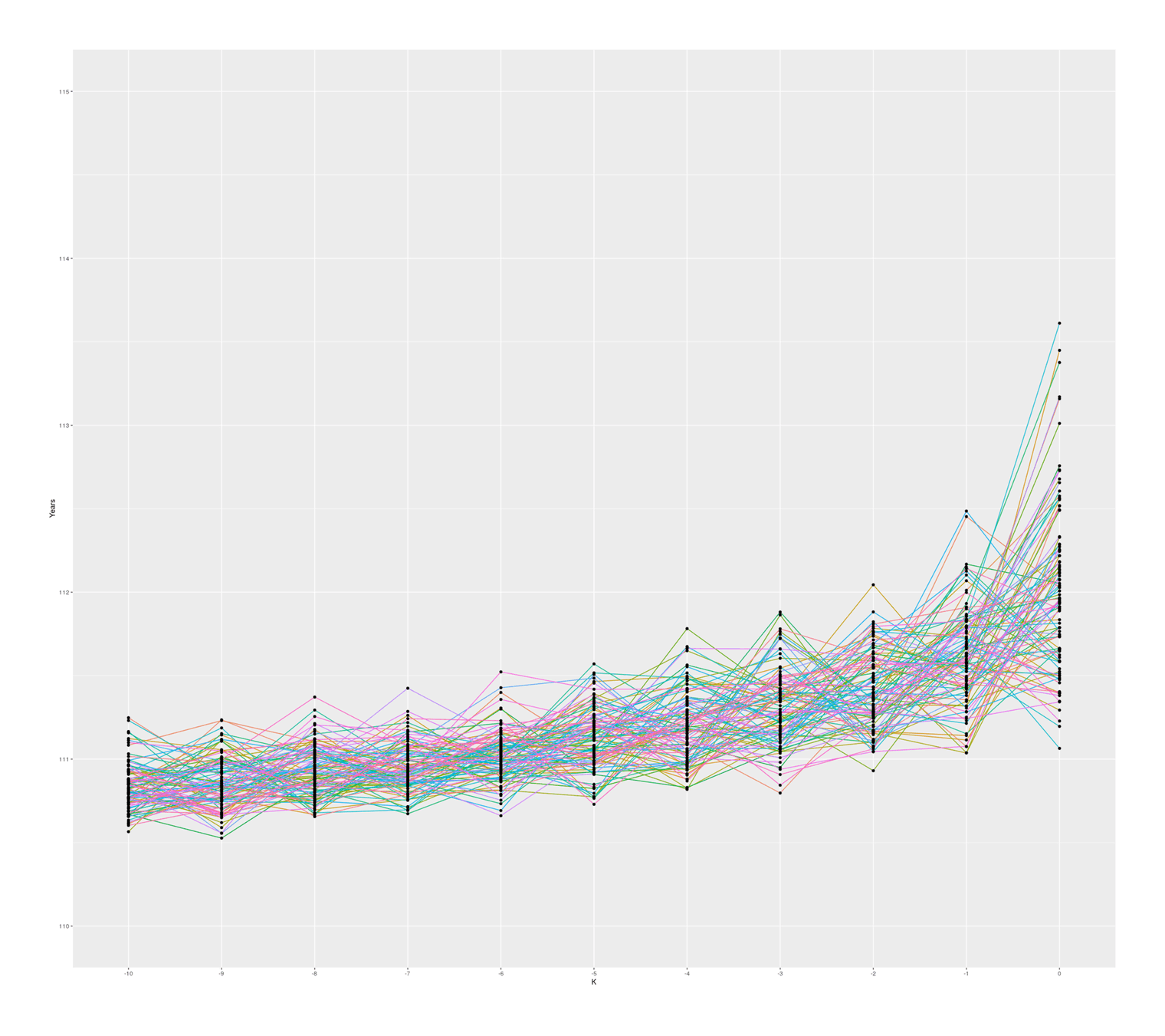
ggplot(small_melted, aes(x = K, y = Years)) +
geom_path(aes(color = V0, group = V0)) + geom_point() +
coord_cartesian(ylim = c(110, 115)) + theme(legend.position = "none")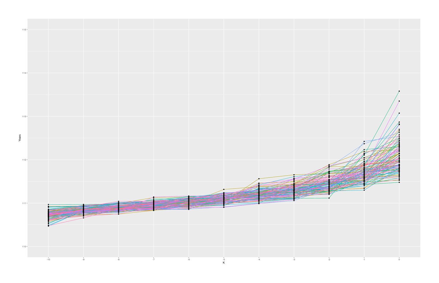
100 simulated samples of top-10-oldest-people out of 10 billion, showing what are reasonable gaps between individuals
With these specific set of parameters, we see median gaps somewhat similar to the empirical data, but we hardly ever (~0.02% of the time) see #1–2 gaps quite as big as Calment’s.
The graph also seems to suggest that there is in fact typically a ‘jump’ between #1 & #2 compared to #2 & #3 and so on, which I was not expecting; thinking about it, I suspect there is some sort of selection effect here: if a random sample from ‘#1’ falls below the random sample of ‘#2’, then they will simply swap places (because when sorted, #2 will be bigger than #1), so an ‘unlucky’ #1 disappears, creating a ratchet effect ensuring the final ‘#1’ will be larger than expected. Any k could exceed expectations, but #1 is the last possible ranking, so it can become more extreme. If I remove the sort call which ensures monotonicity with rank, the graph looks considerably more irregular but still has a jump, so this selection effect may not be the entire story:
100 simulated samples of top-10-oldest-people out of 10 billion; simulated by rank, unsorted (independent samples)
So, overall, a standard Gompertz model does not easily produce a Calment.
This doesn’t prove that the Calment age is wrong, though. It could just be that Calment proves centenarian aging is not well modeled by a Gompertz, or my specific parameter values are wrong (the gaps are similar but the ages are overall off by ~5 years, and perhaps that makes a difference). To begin with, it is unlikely that the Gompertz curve is exactly correct a model of aging; in particular, gerontologists note an apparent ceiling of the annual mortality rate at ~50%, which is inconsistent with the Gompertz (which would continue increasing arbitrarily, quickly hitting >99% annual mortality rates). And maybe Calment really is just an outlier due to sampling error (0.02% ≠ 0%), or she is indeed out of the ordinary human life expectancy distribution but there is a more benign explanation for it like an unique mutation or genetic configuration. But it does seem like Calment’s record is weird in some way.
Sampling Sports Extremes: Hypothetical Human All-Stars League
If we assembled a sports league of the greatest counterfactual athletes from human history, had they all lived in ideal circumstances, how many would be superior to the greatest actual athlete? Not as many as one might think.
As the total human population ever is ~120b and billions have had considerable opportunity, this league couldn’t be >120 in size, as that is how many would be equal to an extreme actual athlete’s rarity (perhaps 1-in-1b).
If we make distributional assumptions like normality, we can calculate the expected number past a threshold like 1-in-1b for 120 replicates; the number is ~77.
In a deleted tweet, the socialist lawyer Matt Bruenig screenshot a block of text to the effect (paraphrasing from memory) that opportunity is denied to most people; consider professional sports—whoever the best athlete in the world is, so few people in history have any opportunity that the ‘missing Einsteins’ (as it’s sometimes phrased by other writers) could probably form an entire pro sports league solely of thousands of athletes better than the best athlete to date.
Is this true? There may be no way to investigate such a claim empirically, but some simple order statistics and demographics can shed some light on it. This ‘hypothetical human all-stars league’ can be reframed as an order statistics question: “what is the expected number of samples from the population of no-opportunity humans which are larger than the observed maximum from the population of had-an-opportunity humans, if we assume some sort of ‘athleticism’ variable and their distributions of this had been identical?”
Is this number plausibly into the thousands? Perhaps surprisingly: no, not without extreme assumptions on either opportunity being drastically more curtailed than it appears to be, or estimates of total human population being wildly wrong. This is because human history is extremely backloaded: thanks to the exponential growth of populations & economies, to a first approximation, most humans have lived recently, and a surprisingly large fraction of all humans to ever live are alive now to enjoy opportunity in a fabulously wealthy world.
First, the total human population throughout human history is usually estimated around only 100–120 billion humans. It is difficult to measure human populations in prehistory, but that is also when the human population of hunter-gatherers must have been tiny, around 0.001b at most; even a lot of error there will not change the bottom line of 120b much, and certainly will not give anything like a 10× increase. We’ll take the high end of 120b, to make the no-opportunity population as large as possible.
Second, the number of people who have opportunity to play professional sports must be a substantial fraction of the current 2022 global population of ~8b. The fact that many countries are not as wealthy as the USA does not mean they lack opportunity. The reach of professional sports is international: baseball players are recruited from the Dominican Republic, Mongolians dominate Japanese sumo wrestling, East African and Caribbean runners outperform in track & field, basketball & hockey stars come from inner cities or all sorts of countries (many ending in ‘-stan’) that one is unfamiliar with, soccer stars come from poor countries like Brazil and grow up in favelas or banlieues, countries recruit shamelessly for their Olympic teams, while even impoverished Communist countries like China or North Korea or the USSR make Olympic competitions a top national priority, lavishly funded to achieve gold at any cost (such as recruiting small children, massive doping programs assisted by intelligence agency covert ops, toleration of systemic sexual abuse, or even rumors of arranged marriages to have tall children like Yao Ming), physical ed and sports are a mandatory part of public schooling (no matter how many concussions kids have), and the public & private investments into sports goes back at least to the original Greek Olympics, when people were poorer than almost anywhere today. Regardless of how impure the motives, or the fact that there is large inequality, it is difficult to look at the resources dedicated to sports in the USA (330m), EU (450m), Japan (125m), Russia (140m), China (1,400m), and come away with any ‘opportunity population’ under 2b for merely the present day—much less throughout history! But let’s be conservative, and make the opportunity population as small as possible, and round it down to 1b.
Comparing Maximum Counts
An easier question to start off with: if there are 120b humans total, and 1b of them had an opportunity, and thus there is some 1 person in that 1b who is ‘the best athlete in the world’ (expected-value of +6.1σ), how many instances would we expect in the 120b were ceteris paribus?
The obvious order statistics answer is just 120 (ie. 119 other than the current one). Because there are 119 other ‘1b units’, and we stipulated they are all the same in terms of potential (would we expect the other 119b to somehow be uniquely superior in potential? why?), so their 1-in-1b sample is identical to our 1-in-1b, and there are 119 of them. This logic works regardless of distribution, we aren’t assuming anything about normality or Gompertz or log-normals here: as long as the distribution is the same, they will all have the same max. It also gives us a quick Fermi estimate for any related questions: simply define the larger population and smaller population, assume their distributions are equal, divide, and that’s the answer.
Right there we can see ‘thousands’ is wrong: there are just too few humans historically, and too much opportunity, to create >1,000 alternative population-units to sample from.4
‘119’ here is not the answer, because we asked about better than, not equal to. But it’s close to the answer as an upper bound: if there are 119 world-athletes as good as our world-athlete, then there can’t be >119 world-athletes better than our world-athlete. There could perhaps be exactly 119 if there was some ceiling of athleticism, but that seems dubious. (There’s not many human abilities where there is a rigid ceiling, and in sports, anytime ceiling effects start hitting, perhaps due to some innovation, the sport will be modified to make it harder and interesting again.) So we could stop here, as the upper bound rules out ‘thousands’, and indicates the number is quite small.
Expected Count Past The Threshold
But if one is curious about how much smaller, exactly, we can keep going. This question requires a distribution: we need to know what the shape of the tail is. If the tail has some sort of truncation-ish shape, then it might be close to 119 but still smaller than 119; if it was something like a Gompertz with a thin tail where the probability drops off incredibly fast, there will be few, perhaps even <1 (but always >0 as long as there is any probability) expected. A normal distribution will be intermediate.
We might be tempted to reuse the code for a truncated normal, but that gives us the expected value of how much better each better all-star player is, not the count of how many better all-star players there are. We can calculate the scenarios we wish with the extreme sampling beta transformation trick as before—just instead of sampling Gompertzs around the Jeanne Calment threshold, we sample normals from a draw of 119b to find how many go past a 1-in-1-billion threshold (+6.1σ) on average.
## What is the expected-value of 1-in-1-billion normals (ie. the threshold)? +6.1σ
exactMax(1e9)
# [1] 6.06946284

## Of 1-in-120b for comparison: +6.8σ (so still quite a gap)
exactMax(1.2e11)
# 6.79682483

## Helper functions from previously:
library(flexsurv)
uk <- function(n, kth, total_n) { rbeta(n, kth, total_n + 1 - kth) }

## Draw from the tail of a normal distribution:
rKNNorm <- function (ie.s, total_n, kth) {
    qnorm(uk(ie.s, kth, total_n), mean=0, sd=1)
    }
simulateSample <- function(total_n, top_k) { sort(sapply(top_k:0,
    function(k) {
        rKNNorm(1, total_n, total_n-k) }
   )) }

## Example: draw the top 10 out of 120b normals:
round(digits=2, simulateSample(1.2e11, 10))
# [1] 6.35 6.36 6.40 6.41 6.45 6.49 6.51 6.59 6.61 6.68 6.76
This looks as expected: the best of 120b is indeed about +6.8σ as the max calculation claimed it should be, and it drops quickly to +6.35σ (thin tails), but the first 10 do not go as low as +6.1σ, in line with the intuition that the true number is ≫0. We could keep simulating more top-k, but simpler to just draw the top 1000 to be safe and count:
## One iteration:
sum(simulateSample(1.2e11, 1000) > exactMax(1e9))
# [1] 80

simulateSamples <- function(total_n, top_k, iters=10000) { t(replicate(ie.s,
    simulateSample(total_n, top_k))) }
simulateSamples(1.2e11, 1000, iters=5)
## 5 examples of a simulation:
round(digits=2, simulateSamples(1.2e11, 100, iters=5))
#      [,1] [,2] [,3] [,4] [,5] [,6] [,7] [,8] [,9] [,10] [,11] [,12] [,13] [,14] [,15] [,16] [,17] [,18] [,19] [,20] [,21] [,22] [,23] [,24] [,25] [,26] [,27] [,28]
# [1,] 6.01 6.01 6.02 6.02 6.03 6.03 6.04 6.04 6.04  6.04  6.04  6.04  6.05  6.05  6.05  6.05  6.05  6.05  6.06  6.06  6.06  6.07  6.07  6.07  6.07  6.07  6.08  6.08
# [2,] 6.02 6.02 6.03 6.03 6.03 6.04 6.04 6.04 6.04  6.04  6.05  6.05  6.05  6.05  6.05  6.05  6.05  6.06  6.06  6.06  6.06  6.07  6.07  6.07  6.08  6.08  6.08  6.08
# [3,] 6.01 6.01 6.02 6.02 6.02 6.03 6.03 6.04 6.04  6.04  6.04  6.04  6.04  6.04  6.05  6.05  6.05  6.05  6.06  6.06  6.06  6.06  6.06  6.06  6.06  6.07  6.07  6.07
# [4,] 5.98 6.02 6.02 6.02 6.03 6.03 6.03 6.04 6.04  6.04  6.05  6.05  6.05  6.05  6.06  6.06  6.06  6.06  6.06  6.06  6.07  6.07  6.07  6.07  6.08  6.08  6.08  6.08
# [5,] 6.00 6.02 6.03 6.04 6.04 6.04 6.04 6.05 6.05  6.05  6.05  6.05  6.05  6.05  6.06  6.06  6.06  6.06  6.06  6.07  6.07  6.07  6.07  6.07  6.07  6.07  6.07  6.07
#      [,29] [,30] [,31] [,32] [,33] [,34] [,35] [,36] [,37] [,38] [,39] [,40] [,41] [,42] [,43] [,44] [,45] [,46] [,47] [,48] [,49] [,50] [,51] [,52] [,53] [,54]
# [1,]  6.08  6.08  6.08  6.08  6.09  6.09  6.09  6.10  6.11  6.11  6.11  6.11  6.11  6.12  6.12  6.12  6.12  6.12  6.12  6.12  6.13  6.13  6.14  6.14  6.14  6.14
# [2,]  6.08  6.09  6.09  6.09  6.09  6.10  6.10  6.10  6.10  6.10  6.11  6.11  6.11  6.12  6.12  6.12  6.13  6.13  6.14  6.14  6.14  6.14  6.14  6.15  6.15  6.16
# [3,]  6.08  6.08  6.08  6.09  6.09  6.10  6.10  6.10  6.10  6.10  6.10  6.10  6.11  6.11  6.11  6.11  6.12  6.12  6.12  6.12  6.13  6.13  6.14  6.14  6.15  6.15
# [4,]  6.08  6.09  6.09  6.09  6.09  6.09  6.09  6.10  6.10  6.10  6.10  6.10  6.11  6.11  6.11  6.11  6.11  6.11  6.12  6.12  6.12  6.12  6.13  6.14  6.15  6.15
# [5,]  6.08  6.08  6.08  6.08  6.08  6.08  6.08  6.08  6.08  6.09  6.10  6.10  6.10  6.10  6.11  6.13  6.13  6.13  6.14  6.14  6.14  6.14  6.14  6.14  6.14  6.14
#      [,55] [,56] [,57] [,58] [,59] [,60] [,61] [,62] [,63] [,64] [,65] [,66] [,67] [,68] [,69] [,70] [,71] [,72] [,73] [,74] [,75] [,76] [,77] [,78] [,79] [,80]
# [1,]  6.14  6.15  6.15  6.15  6.16  6.16  6.16  6.19  6.19  6.19  6.19  6.19  6.19  6.20  6.22  6.23  6.23  6.23  6.24  6.24  6.26  6.26  6.26  6.28  6.28  6.29
# [2,]  6.16  6.16  6.16  6.17  6.17  6.17  6.17  6.17  6.18  6.18  6.19  6.19  6.19  6.19  6.19  6.19  6.20  6.20  6.21  6.23  6.23  6.24  6.24  6.25  6.25  6.26
# [3,]  6.15  6.15  6.15  6.15  6.15  6.15  6.16  6.17  6.18  6.18  6.18  6.19  6.19  6.20  6.21  6.22  6.23  6.23  6.23  6.24  6.25  6.26  6.26  6.28  6.28  6.28
# [4,]  6.15  6.16  6.16  6.16  6.16  6.17  6.17  6.18  6.18  6.18  6.19  6.19  6.19  6.19  6.20  6.20  6.20  6.21  6.22  6.24  6.25  6.25  6.26  6.26  6.28  6.29
# [5,]  6.15  6.15  6.15  6.15  6.16  6.17  6.17  6.18  6.18  6.19  6.20  6.20  6.20  6.20  6.21  6.22  6.22  6.22  6.23  6.23  6.23  6.25  6.25  6.25  6.25  6.25
#      [,81] [,82] [,83] [,84] [,85] [,86] [,87] [,88] [,89] [,90] [,91] [,92] [,93] [,94] [,95] [,96] [,97] [,98] [,99] [,100] [,101]
# [1,]  6.29  6.30  6.30  6.32  6.33  6.33  6.34  6.36  6.37  6.38  6.39  6.43  6.43  6.46  6.50  6.51  6.52  6.56  6.61   6.72   6.96
# [2,]  6.27  6.27  6.27  6.31  6.31  6.31  6.32  6.32  6.34  6.35  6.37  6.41  6.41  6.43  6.46  6.46  6.52  6.60  6.64   6.81   6.83
# [3,]  6.29  6.30  6.30  6.31  6.33  6.34  6.35  6.35  6.36  6.40  6.41  6.42  6.44  6.46  6.49  6.58  6.61  6.67  6.68   6.73   6.76
# [4,]  6.29  6.29  6.30  6.30  6.32  6.33  6.34  6.34  6.36  6.36  6.42  6.44  6.44  6.44  6.45  6.47  6.54  6.54  6.60   6.69   6.76
# [5,]  6.27  6.28  6.30  6.30  6.31  6.32  6.32  6.33  6.38  6.39  6.41  6.43  6.45  6.48  6.52  6.57  6.57  6.61  6.61   6.66   7.03

## 10k iterations to be safe:
replicate(1000, sum(simulateSample(1.2e11, 1000) > exactMax(1e9)))
#   [1] 76 76 79 75 77 76 79 76 81 77 72 76 80 81 75 81 80 78 79 80 75 79 81 74 79 76 77 79 72 73 78 76 77 78 75 78 78 76 73 81 76 78 80 78 78 80 78 79 74 74 80 77 77
#  [54] 73 76 81 78 79 76 75 76 77 76 79 78 79 76 82 76 78 77 76 81 84 81 76 76 80 77 79 74 76 78 78 78 76 74 76 76 76 80 79 77 77 76 77 77 77 75 73 79 74 79 80 75 76
# [107] 76 80 76 76 74 78 80 76 78 75 75 75 75 76 76 77 74 75 78 79 78 80 81 75 76 76 75 76 76 78 79 80 78 78 76 79 78 77 77 74 78 79 77 79 76 75 74 73 75 77 76 80 75
# [160] 79 76 74 75 76 78 76 75 77 78 79 78 76 75 79 77 79 79 76 82 75 79 78 73 79 76 77 78 79 78 75 76 74 74 78 75 77 77 77 74 76 77 76 75 79 80 76 76 75 81 75 77 76
# [213] 79 74 77 77 77 81 80 81 79 78 75 79 80 77 81 79 78 79 74 74 75 76 80 77 78 79 77 74 79 78 80 75 77 79 80 72 75 74 78 79 78 81 75 74 80 77 78 78 78 81 77 80 77
# [266] 79 75 81 77 77 77 73 75 75 76 80 77 75 80 77 75 79 76 76 81 72 78 76 79 76 78 79 77 81 75 77 77 78 80 75 75 78 73 77 77 79 78 82 75 74 82 80 79 74 78 79 78 77
# [319] 75 74 78 76 76 75 75 74 79 78 76 75 77 78 79 81 75 76 76 77 80 79 75 74 83 76 74 75 77 76 78 75 79 79 75 81 80 77 76 76 78 80 77 73 79 77 79 75 76 80 76 81 79
# [372] 80 73 74 77 80 73 77 77 74 77 76 80 76 73 77 81 73 76 76 81 79 76 74 77 74 76 79 77 77 78 77 77 78 77 78 80 79 77 72 73 77 75 79 80 78 78 79 79 79 77 77 81 74
# [425] 77 79 71 75 80 73 74 78 77 75 75 73 77 75 77 78 78 80 76 74 78 77 76 75 76 79 79 77 78 80 77 80 80 78 78 75 75 79 80 79 77 80 83 77 78 76 74 81 78 77 79 79 79
# [478] 74 76 74 75 75 75 82 78 76 80 76 77 78 76 78 77 78 79 76 76 79 75 80 74 74 72 77 77 79 77 79 78 75 82 72 80 75 79 79 77 78 78 76 75 79 77 76 76 77 75 81 75 76
# [531] 78 77 79 75 78 78 75 76 80 76 75 77 79 77 76 78 79 78 79 78 73 74 78 77 79 75 75 79 77 78 74 83 76 79 77 80 81 79 77 81 75 79 78 76 73 78 77 74 80 77 78 78 75
# [584] 77 78 78 77 73 76 79 75 80 77 78 77 78 77 75 80 76 81 78 78 81 79 74 81 76 81 79 76 78 78 79 76 77 75 77 76 78 79 76 78 77 75 77 73 76 77 76 81 78 73 76 77 76
# [637] 80 80 78 79 76 78 77 78 78 76 80 77 74 75 77 75 76 76 75 78 76 78 75 75 75 73 74 75 72 79 75 78 78 78 76 80 79 78 81 74 74 80 77 77 78 73 77 73 75 76 81 77 78
# [690] 76 77 75 79 78 74 74 73 76 81 77 73 77 76 76 78 77 75 79 77 77 77 77 78 76 76 80 76 75 76 77 76 77 74 74 77 78 77 76 75 78 77 81 72 81 79 76 74 77 80 75 77 82
# [743] 74 76 75 74 76 79 75 78 77 81 74 78 77 76 77 83 78 79 78 80 76 75 78 71 82 76 75 77 78 80 75 75 79 80 75 77 74 79 77 77 74 76 72 75 77 80 78 75 79 76 75 79 85
# [796] 77 75 77 76 79 79 77 80 74 76 75 77 77 78 77 76 76 74 80 76 76 78 77 76 78 78 73 79 78 82 78 81 80 80 77 79 77 80 79 79 73 76 78 78 74 77 81 81 77 77 76 78 76
# [849] 76 79 76 78 76 82 77 82 77 76 74 79 74 78 73 78 74 76 83 76 81 75 77 79 81 77 77 77 76 75 78 78 78 79 77 80 77 76 77 77 76 77 80 76 73 78 76 77 76 77 78 78 75
# [902] 77 76 77 80 75 77 83 79 74 80 74 78 79 78 73 80 79 76 76 73 76 75 77 76 78 77 77 77 73 77 76 77 76 76 78 76 74 76 75 77 78 80 76 76 75 76 76 74 81 73 74 75 74
# [955] 77 78 74 78 79 75 82 77 75 79 78 82 75 73 78 77 82 79 75 73 76 77 75 71 79 82 74 80 77 78 76 75 78 79 77 76 77 79 79 75 76 75 75 81 78 76

## Mean:
mean(replicate(1000, sum(simulateSample(1.2e11, 1000) > exactMax(1e9))))
# [1] 77.075

## What if we shrink opportunity by an order of magnitude?
sum(simulateSample(1.2e11, 1000) > exactMax(1e8))
# [1] 770
So the upper bound was loose by about a third: we actually get ~77 all-star league players. This is also robust: even dropping opportunity by (another) order of magnitude still doesn’t get near 1,000, much less thousands.
Exploiting the beta transformation, where the order statistics of a simple 0–1 interval turns out to follow a beta distribution (specifically: U(k) ~ Beta(k, n + 1 − k)), which can then be easily transformed into the equivalent order statistics of more useful distributions like the normal distribution. The beta transformation is not just computationally useful, but critical to order statistics in general.↩︎
lmomcois accurate for all values I checked with Monte Carlo n < 1000, but appears to have some bugs n > 200026ya: there are occasional deviations from the quasi-logarithmic curve, such as n = 2225–2236 (which are off by 1.02SD compared to the Monte Carlo estimates and the surrounding lmomco estimates), another cluster of errors n ~ 40,000, and then after n > 60,000, the estimates are incorrect. The maintainer has been notified & verified the bug.↩︎A previous version of
EnvStatsdescribed the approximation thus:
↩︎The function
evNormOrdStatsScalarcomputes the value of 𝔼(r,n) for user-specified values of r and n. The functionevNormOrdStatscomputes the values of 𝔼(r,n) for all values of r for a user-specified value of n. For large values of n, the functionevNormOrdStatswithapproximate=FALSEmay take a long time to execute. Whenapproximate=TRUE,evNormOrdStatsandevNormOrdStatsScalaruse the following approximation to 𝔼(r,n), which was proposed by Blom (195868ya, pp. 68–75, [“6.9 An approximate mean value formula” & formula 6.10.3–6.10.5]):## General Blom 1958 approximation: blom1958E <- function(r,n) { qnorm((r - 3/8) / (n + 1/4)) } blom1958E(10^10, 10^10) # [1] 6.433133208This approximation is quite accurate. For example, for n ≥ 2, the approximation is accurate to the first decimal place, and for n ≥ 9 it is accurate to the second decimal place.
If we don’t mess with 120b, to fit >1,000, we’d have to cut the units down in size to <0.12b each, which is absurd—if we imagined no one dead ever had any opportunity & only the living ever got an opportunity, that’d still mean <2% of the global population ever ‘had an opportunity’!↩︎