Anthology of sociology, statistical, or psychological papers discussing the observation that all real-world variables have non-zero correlations and the implications for statistical theory such as ‘null hypothesis testing’.
Statistical folklore asserts that “everything is correlated”: in any real-world dataset, most or all measured variables will have non-zero correlations, even between variables which appear to be completely independent of each other, and that these correlations are not merely sampling error flukes but will appear in large-scale datasets to arbitrarily designated levels of statistical-significance or posterior probability.
This raises serious questions for null-hypothesis statistical-significance testing, as it implies the null hypothesis of 0 will always be rejected with sufficient data, meaning that a failure to reject only implies insufficient data, and provides no actual test or confirmation of a theory. Even a directional prediction is minimally confirmatory since there is a 50% chance of picking the right direction at random.
It also has implications for conceptualizations of theories & causal models, interpretations of structural models, and other statistical principles such as the “sparsity principle”.
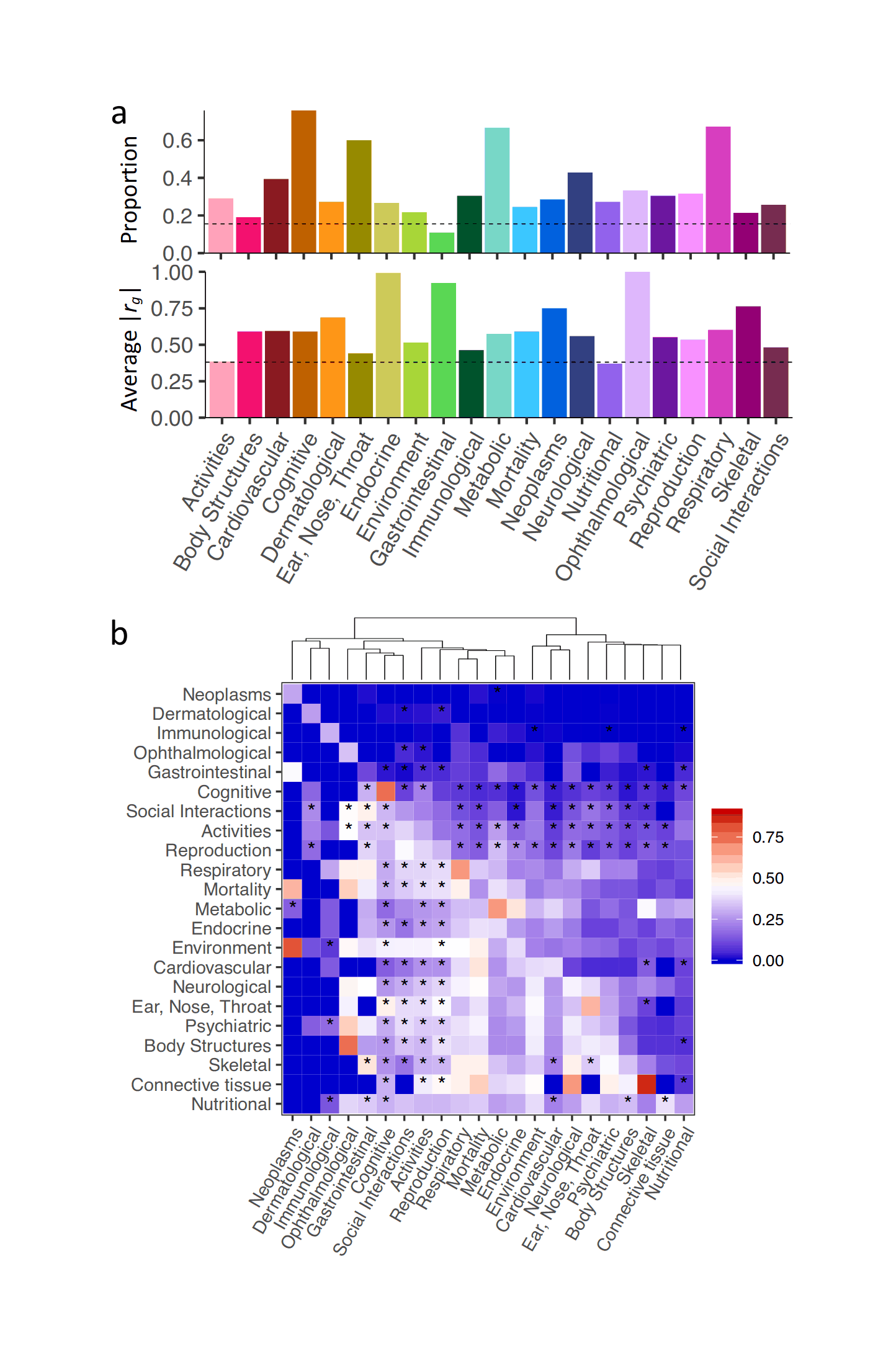
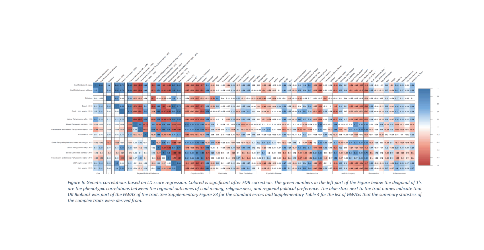
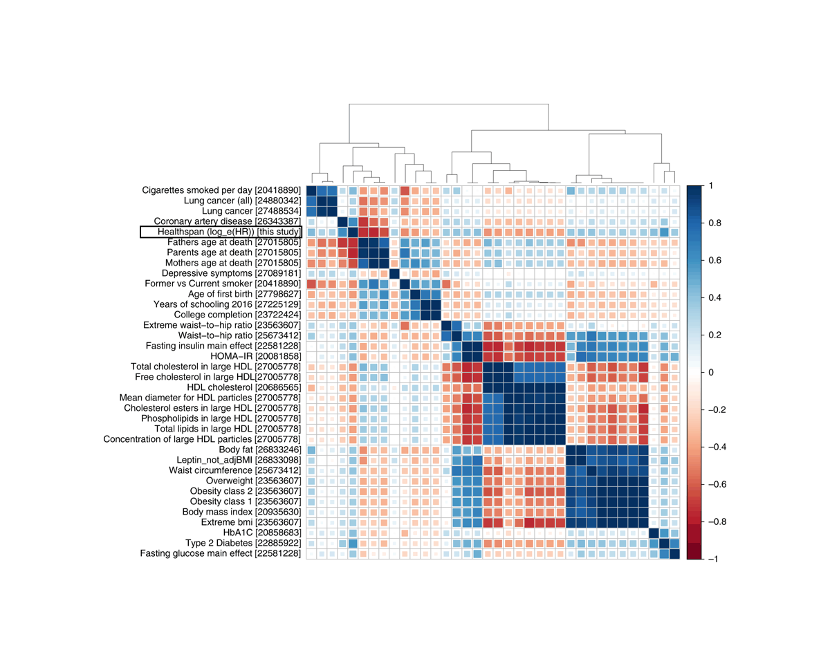
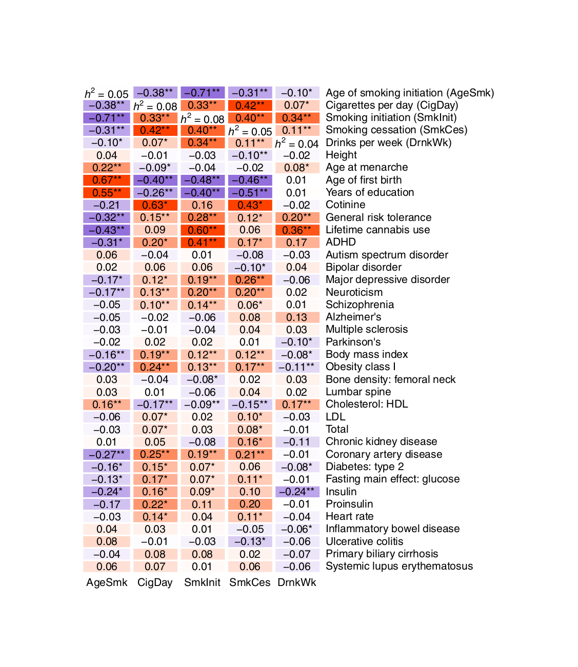
The core idea here is that in any real-world dataset, it is exceptionally unlikely that any particular relationship will be exactly 0 for reasons of arithmetic (eg. it may be impossible for a binary variable to be an equal percentage in 2 unbalanced groups); prior probability (0 is only one number out of the infinite reals); and because real-world properties & traits are linked by a myriad of causal networks, dynamics, & latent variables (eg. the genetic correlations which affect all human traits, see heat maps in appendix for visualizations) which mutually affect each other which will produce genuine correlations between apparently-independent variables, and these correlations may be of surprisingly large & important size.
These reasons are unaffected by sample size and are not simply due to ‘small n’. If we simulate out uncorrelated random variables, even with small sizes, they quickly approach absolute correlations of ~0, and few will be of meaningful size like |r| > 0.10:
# Simulation of the 'crud factor' in psychology, where variables seem to always be intercorrelated non-zero, with a rough absolute correlation of 0.1.# I would like to simulate out the null hypothesis of completely uncorrelated variables in plausible dataset sizes.# So this is a R Monte Carlo simulation to simulate a multivariate normal distribution of 1,000 independent, uncorrelated N(0,1) variables and drawing 1,000 datapoints from it; calculate the sample r correlation of all the variables, and what fraction are correlated r > |0.1|. Then let's Monte Carlo that, say, 100 times (to avoid taking too long) and plot the averaged distributions of the |r| histogram.# Output:# # Mean proportion of |r| > 0.1: 0.002 (SD: 0.000)library(MASS)library(ggplot2)library(reshape2)library(parallel)# Parametersn_vars <-1000n_samples <-1000n_sims <-100threshold <-0.1# Function to run one simulation and return correlation metricsrun_simulation <-function(seed, n_vars, n_samples, threshold) {set.seed(seed) sigma <-diag(n_vars) data <-mvrnorm(n = n_samples,mu =rep(0, n_vars),Sigma = sigma) cors <-cor(data) cors_upper <- cors[upper.tri(cors)]# Return both the histogram counts and proportion above threshold hist_data <-hist(abs(cors_upper), breaks =seq(0, 1, by =0.01), plot =FALSE)return(list(hist_counts = hist_data$counts,prop_above_thresh =mean(abs(cors_upper) > threshold) ))}# Set up parallel processingn_cores <-detectCores() -1cl <-makeCluster(n_cores)# Export required packages and variables to the clusterclusterEvalQ(cl, {library(MASS)})clusterExport(cl, c("n_vars", "n_samples", "threshold"))# Run simulations in parallelseeds <-1:n_simsresults <-parLapply(cl, seeds, run_simulation,n_vars = n_vars,n_samples = n_samples,threshold = threshold)# Clean upstopCluster(cl)# Process resultsprops <-sapply(results, function(x) x$prop_above_thresh)mean_prop <-mean(props)# Average the histogram counts across simulationsavg_counts <-Reduce('+', lapply(results, function(x) x$hist_counts)) / n_sims# Calculate total possible correlations for one simulationtotal_cors <- (n_vars * (n_vars -1)) /2# Create plotting dataplot_data <-data.frame(correlation =seq(0, 0.99, by =0.01)[1:length(avg_counts)],count = avg_counts)# Create histogramp1 <-ggplot(plot_data, aes(x = correlation, y = count/total_cors *100)) +geom_bar(stat ="identity", fill ="blue", alpha =0.7) +theme_bw(base_size =40) +geom_vline(xintercept = threshold, color ="red", linetype ="dashed", size=3) +theme(plot.title =element_text(face ="bold")) +scale_y_continuous(labels =function(x) paste0(round(x, 1), "%"),name ="Percentage of All Inter-Correlations",expand =c(0, 0),limits =c(0, NA) ) +scale_x_continuous(name =expression(paste("Absolute Correlation (|", italic("r"), "|)")),breaks =seq(0, 0.13, by =0.02),expand =c(0, 0),limits =c(0, 0.13) ) +annotate("text",x =0.101,y =max(avg_counts/total_cors *100)/3,label =substitute(paste(value, "% exceed |", italic("r"), "| > ", thresh),list(value =sprintf("%.1f", 100* mean_prop),thresh =sprintf("%.2f", threshold))),size =10,hjust =0) +labs(title ="Distribution of Absolute Correlations")# Print summary statisticscat(sprintf("Mean proportion of |r| > 0.1: %.3f (SD: %.3f)\n", mean(props), sd(props)))print(p1)
A Monte Carlo simulation of an uncorrelated multivariate normal in R shows that even with p = 1,000 and n = 1,000 (many variables and a small dataset), we rarely will observe ‘crud factor’-style correlations between uncorrelated variables, and so the crud factor is not a statistical triviality.
The claim is generally backed up by personal experience and reasoning, although in a few instances like Meehl large datasets are mentioned in which almost all variables are correlated at high levels of statistical-significance.
Sharp null hypotheses are meaningless: The most commonly mentioned, and the apparent motivation for early discussions, is that in the null-hypothesis significance-testing paradigm dominant in psychology and many sciences, any sharp null-hypothesis such as a parameter (like a Pearson’s r correlation) being exactly equal to 0 is known—in advance—to already be false and so it will inevitably be rejected as soon as sufficient data collection permits sampling to the foregone conclusion.
The existence of pervasive correlations, in addition to the presence of systematic error4, guarantees nonzero ‘effects’. This renders the meaning of significance-testing unclear; it is calculating precisely the odds of the data under scenarios known a priori to be false.
Directional hypotheses are little better: better null-hypotheses, such as >0 or <0, are also problematic since if the true value of a parameter is never 0 then one’s theories have at least a 50-50 chance of guessing the right direction and so correct ‘predictions’ of the sign count for little.
This renders any successful predictions of little value.
Model interpretation is difficult: This extensive intercorrelation threatens many naive statistical models or theoretical interpretations thereof, quite aside from p-values
For example, given the large amounts of measurement error in most sociological or psychological traits such as SES, home environment, or IQ, fully ‘controlling for’ a latent variable based on measured variables is difficult or impossible and said variable will in fact be correlated with the primary variable of interest, leading to “residual confounding”
The existence of both “everything is correlated” and the success of the “bet on sparsity” principle suggests that these causal networks may be best thought of as having hubs or latent variables: there are a relatively few variables such as ‘arousal’ or ‘IQ’ which play central roles, explaining much of variance, followed by almost all other variables accounting for a little bit each with most of their influence mediated through the key variables.
The fact that these variables can be successfully modeled as substantively linear or additive further implies that interactions between variables will be typically rare or small or both (implying further that most such hits will be false positives, as interactions are already harder to detect than main effects, and more so if they are a priori unlikely or of small size). Even extremely large & deeply phenotyped datasets may struggle to achieve impressive improvements over baselines using the core variables (eg. Salganik et al 2020).
To the extent that these key variables are unmodifiable, the many peripheral variables may also be unmodifiable (which may be related to the broad failure of social intervention programs). Any intervention on those peripheral variables, being ‘downstream’, will tend to either be ‘hollow’ or fade out or have no effect at all on the true desired goals no matter how consistently they are correlated.
On a more contemporary note, these theoretical & empirical considerations also throw doubt on concerns about ‘algorithmic bias’ or inferences drawing on ‘protected classes’: not drawing on them may not be desirable, possible, or even meaningful.
Uncorrelated variables may be meaningless: given this empirical reality, any variable which is uncorrelated with the major variables is suspicious (somewhat like the pervasiveness of heritability in human traits renders traits with zero heritability suspicious, suggesting issues like measuring at the wrong time). The lack of correlation suggests that the analysis is underpowered, something has gone wrong in the construction of the variable/dataset, or that the variable is part of a system whose causal network renders conventional analyses dangerously misleading.
For example, the dataset may be corrupted by a systematic bias such as range restriction or a selection effect such as Simpson’s paradox, which erases from the data a correlation that actually exists. Or the data may be random noise, due to software error or fraud or extremely high levels of measurement error (such as “lizardman constant” respondents answering at random); or the variable may not be real in the first place. Another possibility is that the variable is causally connected, in feedback loops (especially common in economics or biology), to another variable, in which case the standard statistical machinery is misleading—the classic example is Milton Friedman’s thermostat, noting that a thermostat would be almost entirely uncorrelated with room temperature.
This idea, as suggested by the many names, is not due to any single theoretical or empirical result or researcher, but has been made many times by many different researchers in many contexts, circulating as informal ‘folklore’. To bring some order to this, I have compiled excerpts of some relevant references in chronological order. (Additional citations are welcome.)
In early November 1904122ya, Gosset discussed his first breakthrough in an internal report entitled “The Application of the ‘Law of Error’ to the Work of the Brewery” (Gosset 1904122ya; Laboratory Report, Nov. 3, 1904122ya, pg3). Gosset (p. 3–16) wrote:
Results are only valuable when the amount by which they probably differ from the truth is so small as to be insignificant for the purposes of the experiment. What the odds should be depends
On the degree of accuracy which the nature of the experiment allows, and
On the importance of the issues at stake.
Two features of Gosset’s report are especially worth highlighting here. First, he suggested that judgments about “significant” differences were not a purely probabilistic exercise: they depend on the “importance of the issues at stake.” Second, Gosset underscored a positive correlation in the normal distribution curve between “the square root of the number of observations” and the level of statistical-significance. Other things equal, he wrote, “the greater the number of observations of which means are taken [the larger the sample size], the smaller the [probable or standard] error” (pg5). “And the curve which represents their frequency of error”, he illustrated, “becomes taller and narrower” (pg7).
Since its discovery in the early 19th century, tables of the normal probability curve had been created for large samples…The relation between sample size and “significance” was rarely explored. For example, while looking at biometric samples with up to thousands of observations, Karl Pearson declared that a result departing by more than 3 standard deviations is “definitely significant.”12 Yet Gosset, a self-trained statistician, found that at such large samples, nearly everything is statistically “significant”—though not, in Gosset’s terms, economically or scientifically “important.” Regardless, Gosset didn’t have the luxury of large samples. One of his earliest experiments employed a sample size of 2 (Gosset, 1904122ya, p.7) and in fact in “The Probable Error of a Mean” he calculated a t statistic for n = 2 (Student, 1908118yab, p. 23).
…the “degree of certainty to be aimed at”, Gosset wrote, depends on the opportunity cost of following a result as if true, added to the opportunity cost of conducting the experiment itself. Gosset never deviated from this central position.15 [See, for example, Student (1923, p. 271, paragraph one: “The object of testing varieties of cereals is to find out which will pay the farmer best.”) and Student (1931c, p. 1342, paragraph one) reprinted in Student (194284ya, p. 90 and p. 150).]
…the significance of intelligence for success in a given activity of life is measured by the coefficient of correlation between them. Scientific investigations of these matters is just beginning; and it is a matter of great difficulty and expense to measure the intelligence of, say, a thousand clergymen, and then secure sufficient evidence to rate them accurately for their success as ministers of the Gospel. Consequently, one can report no final, perfectly authoritative results in this field. One can only organize reasonable estimates from the various partial investigations that have been made. Doing this, I find the following:
Intelligence and success in the elementary schools, r = +0.80
Intelligence and success in high-school and colleges in the case of those who go, r = +0.60; but if all were forced to try to do this advanced work, the correlation would be +0.80 or more.
Intelligence and salary, r = +0.35.
Intelligence and success in athletic sports, r = +0.25
Intelligence and character, r = +0.40
Intelligence and popularity, r = +0.20
Whatever be the eventual exact findings, two sound principles are illustrated by our provisional list. First, there is always some resemblance; intellect always counts. Second, the resemblance varies greatly; intellect counts much more in some lines than in others.
The first fact is in part a consequence of a still broader fact or principle—namely, that in human nature good traits go together. To him that hath a superior intellect is given also on the average a superior character; the quick boy is also in the long run more accurate; the able boy is also more industrious. There is no principle of compensation whereby a weak intellect is offset by a strong will, a poor memory by good judgment, or a lack of ambition by an attractive personality. Every pair of such supposed compensating qualities that have been investigated has been found really to show correspondence. Popular opinion has been misled by attending to striking individual cases which attracted attention partly because they were really exceptions to the rule. The rule is that desirable qualities are positively correlated. Intellect is good in and of itself, and also for what it implies about other traits.
I believe that an observant statistician who has had any considerable experience with applying the chi-square test repeatedly will agree with my statement that, as a matter of observation, when the numbers in the data are quite large, the P’s tend to come out small. Having observed this, and on reflection, I make the following dogmatic statement, referring for illustration to the normal curve: “If the normal curve is fitted to a body of data representing any real observations whatever of quantities in the physical world, then if the number of observations is extremely large—for instance, on an order of 200,000—the chi-square P will be small beyond any usual limit of significance.”
This dogmatic statement is made on the basis of an extrapolation of the observation referred to and can also be defended as a prediction from a priori considerations. For we may assume that it is practically certain that any series of real observations does not actually follow a normal curve with absolute exactitude in all respects, and no matter how small the discrepancy between the normal curve and the true curve of observations, the chi-square P will be small if the sample has a sufficiently large number of observations in it.
If this be so, then we have something here that is apt to trouble the conscience of a reflective statistician using the chi-square test. For I suppose it would be agreed by statisticians that a large sample is always better than a small sample. If, then, we know in advance the P that will result from an application of a chi-square test to a large sample, there would seem to be no use in doing it on a smaller one. But since the result of the former test is known, it is no test at all.
Your City, Thorndike 193987ya (and the followup 144 Smaller Cities providing tables for 144 cities) compiles various statistics about American cities such as infant mortality, spending on the arts, crime etc. and finds extensive intercorrelations & factors.
The general factor of socioeconomic status or ‘S-factor’ also applies across countries as well: economic growth is by far the largest influence on all measures of well-being, and attempts at computing international rankings of things like maternal founder on this fact, as they typically wind up simply reproducing GDP rank-orderings and being redundant. For example, Jones & Klenow 2016 compute an international wellbeing metric using “life expectancy, the ratio of consumption to income, annual hours worked per capita, the standard deviation of log consumption, and the standard deviation of annual hours worked” to incorporate factors like inequality, but this still winds up just being equivalent to GDP (r = 0.98). Or Gill & Gebhart 2016, who note that of 9 international indices they consider, all correlate positively with per capita GDP, & 6 have rank-correlations τ > 0.5.
The general question of significance tests was raised in 7.3 and a simple example will now be considered. Suppose that a die is thrown n times and that it shows an r-face on mr occasions (r = 1, 2, …, 6). The question is whether the die is loaded. The answer depends on the meaning of “loaded”. From one point of view, it is unnecessary to look at the statistics since it is obvious that no die could be absolutely symmetrical. [It would be no contradiction of 4.3 (2) to say that the hypothesis that the die is absolutely symmetrical is almost impossible. In fact, this hypothesis is an idealised proposition rather than an empirical one.] It is possible that a similar remark applies to all experiments—even to the ESP experiment, since there may be no way of designing it so that the probabilities are exactly equal to 1⁄2.
When testing statistical hypotheses, we usually do not wish to take the action of rejection unless the hypothesis being tested is false to an extent sufficient to matter. For example, we may formulate the hypothesis that a population is normally distributed, but we realize that no natural population is ever exactly normal. We would want to reject normality only if the departure of the actual distribution from the normal form were great enough to be material for our investigation. Again, when we formulate the hypothesis that the sex ratio is the same in two populations, we do not really believe that it could be exactly the same, and would only wish to reject equality if they are sufficiently different. Further examples of the phenomenon will occur to the reader.
The development of the theory of testing has been much influenced by the special problem of simple dichotomy, that is, testing problems in which H0 and H1 have exactly one element each. Simple dichotomy is susceptible of neat and full analysis (as in Exercise 7.5.2 and in §14.4), likelihood-ratio tests here being the only admissible tests; and simple dichotomy often gives insight into more complicated problems, though the point is not explicitly illustrated in this book.
Coin and ball examples of simple dichotomy are easy to construct, but instances seem rare in real life. The astronomical observations made to distinguish between the Newtonian and Einsteinian hypotheses are a good, but not perfect, example, and I suppose that research in Mendelian genetics sometimes leads to others. There is, however, a tradition of applying the concept of simple dichotomy to some situations to which it is, to say the best, only crudely adapted. Consider, for example, the decision problem of a person who must buy, f0, or refuse to buy, f1, a lot of manufactured articles on the basis of an observation x. Suppose that i is the difference between the value of the lot to the person and the price at which the lot is offered for sale, and that P(x | i) is known to the person. Clearly, H0, H1, and N are sets characterized respectively by i > 0, i < 0, i = 0. This analysis of this, and similar, problems has recently been explored in terms of the minimax rule, for example by Sprowls [S16] and a little more fully by Rudy [R4], and by Allen [A3]. It seems to me natural and promising for many fields of application, but it is not a traditional analysis. On the contrary, much literature recommends, in effect, that the person pretend that only two values of i, i0 > 0 and i1 < 0, are possible and that the person then choose a test for the resulting simple dichotomy. The selection of the two values i0 and i1 is left to the person, though they are sometimes supposed to correspond to the person’s judgment of what constitutes good quality and poor quality—terms really quite without definition. The emphasis on simple dichotomy is tempered in some acceptance-sampling literature, where it is recommended that the person choose among available tests by some largely unspecified overall consideration of operating characteristics and costs, and that he facilitate his survey of the available tests by focusing on a pair of points that happen to interest him and considering the test whose operating characteristic passes (economically, in the case of sequential testing) through the pair of points. These traditional analyses are certainly inferior in the theoretical framework of the present discussion, and I think they will be found inferior in practice.
…I turn now to a different and, at least for me, delicate topic in connection with applications of the theory of testing. Much attention is given in the literature of statistics to what purport to be tests of hypotheses, in which the null hypothesis is such that it would not really be accepted by anyone. The following 3 propositions, though playful in content, are typical in form of these extreme null hypotheses, as I shall call them for the moment.
A. The mean noise output of the cereal Krakl is a linear function of the atmospheric pressure, in the range 900–1,100 millibars. B. The basal metabolic consumption of sperm whales is normally distributed [White et al 1953]. C. New York taxi drivers of Irish, Jewish, and Scandinavian extraction are equally proficient in abusive language.
Literally to test such hypotheses as these is preposterous. If, for example, the loss associated with f1 is zero, except in case Hypothesis A is exactly satisfied, what possible experience with Krakl could dissuade you from adopting f1?
The unacceptability of extreme null hypotheses is perfectly well known; it is closely related to the often heard maxim that science disproves, but never proves, hypotheses. The role of extreme hypotheses in science and other statistical activities seems to be important but obscure. In particular, though I, like everyone who practices statistics, have often “tested” extreme hypotheses, I cannot give a very satisfactory analysis of the process, nor say clearly how it is related to testing as defined in this chapter and other theoretical discussions. None the less, it seems worth while to explore the subject tentatively; I will do so largely in terms of two examples.
Consider first the problem of a cereal dynamicist who must estimate the noise output of Krakl at each of 10 atmospheric pressures between 900 and 1,100 millibars. It may well be that he can properly regard the problem as that of estimating the 10 parameters in question, in which case there is no question of testing. But suppose, for example, that one or both of the following considerations apply. First, the engineer and his colleagues may attach considerable personal probability to the possibility that A is very nearly satisfied—very nearly, that is, in terms of the dispersion of his measurements. Second, the administrative, computational, and other incidental costs of using 10 individual estimates might be considerably greater than that of using a linear formula.
It might be impractical to deal with either of these considerations very rigorously. One rough attack is for the engineer first to examine the observed data x and then to proceed either as though he actually believed Hypothesis A or else in some other way. The other way might be to make the estimate according to the objectivistic formulae that would have been used had there been no complicating considerations, or it might take into account different but related complicating considerations not explicitly mentioned here, such as the advantage of using a quadratic approximation. It is artificial and inadequate to regard this decision between one class of basic acts or another as a test, but that is what in current practice we seem to do. The choice of which test to adopt in such a context is at least partly motivated by the vague idea that the test should readily accept, that is, result in acting as though the extreme null hypotheses were true, in the farfetched case that the null hypothesis is indeed true, and that the worse the approximation of the null hypotheses to the truth the less probable should be the acceptance.
The method just outlined is crude, to say the best. It is often modified in accordance with common sense, especially so far as the second consideration is concerned. Thus, if the measurements are sufficiently precise, no ordinary test might accept the null hypotheses, for the experiment will lead to a clear and sure idea of just what the departures from the null hypotheses actually are. But, if the engineer considers those departures unimportant for the context at hand, he will justifiably decide to neglect them.
Rejection of an extreme null hypothesis, in the sense of the foregoing discussion, typically gives rise to a complicated subsidiary decision problem. Some aspects of this situation have recently been explored, for example by Paulson 1949, Paulson 1952; Duncan 195175ya, Duncan 195274ya; Tukey 194977ya, Tukey 195175ya; Scheffe 1953; and Walter D. Fisher 1953.
…However, the calculation [of error rates of ‘rejecting the null’] is absurdly academic, for in fact no scientific worker has a fixed level of significance at which from year to year and in all circumstances, he rejects hypotheses; he rather gives his mind to each particular case in the light of his evidence and his ideas. Further, the calculation is based solely on a hypothesis, which, in the light of the evidence, is often not believed to be true at all, so that the actual probability of erroneous decision, supposing such a phrase to have any meaning, may be much less than the frequency specifying the level of significance.
A difficulty with this viewpoint is that it is often known that the hypothesis tested could not be precisely true. No coin, for example, has a probability of precisely 1⁄2 of coming heads. The true probability will always differ from 1⁄2 even if it differs by only 0.000,000,000,1. Neither will any treatment cure precisely one-third of the patients in the population to which it might be applied, nor will the proportion of voters in a presidential election favoring one candidate be precisely1⁄2. Recognition of this leads to the notion of differences that are or are not of practical importance. “Practical importance” depends on the actions that are going to be taken on the basis of the data, and on the losses from taking certain actions when others would be more appropriate.
Thus, the focus is shifted to decisions: Would the same decision about practical action be appropriate if the coin produces heads 0.500,000,000,1 of the time as if it produces heads 0.5 of the time precisely? Does it matter whether the coin produces heads 0.5 of the time or 0.6 of the time, and if so does it matter enough to be worth the cost of the data needed to decide between the actions appropriate to these situations? Questions such as these carry us toward a comprehensive theory of rational action, in which the consequences of each possible action are weighed in the light of each possible state of reality. The value of a correct decision, or the costs of various degrees of error, are then balanced against the costs of reducing the risks of error by collecting further data. It is this viewpoint that underlies the definition of statistics given in the first sentence of this book. [“Statistics is a body of methods for making wise decisions in the face of uncertainty.”]
Siegel does not explain why his interest is confined to tests of significance; to make measurements and then ignore their magnitudes would ordinarily be pointless. Exclusive reliance on tests of significance obscures the fact that statistical-significance does not imply substantive significance. The tests given by Siegel apply only to null hypotheses of “no difference.” In research, however, null hypotheses of the form “Population A has a median at least 5 units larger than the median of Population B” arise. Null hypotheses of no difference are usually known to be false before the data are collected [9, p. 42; 48, pp. 384–8]; when they are, their rejection or acceptance simply reflects the size of the sample and the power of the test, and is not a contribution to science.
The most misused and misconceived hypothesis-testing model employed in psychology is referred to as the “null-hypothesis” model. Stating it crudely, one null hypothesis would be that two treatments do not produce different mean effects in the long run. Using the obtained means and sample estimates of”population” variances, probability statements can be made about the acceptance or rejection of the null hypothesis. Similar null hypotheses are applied to correlations, complex experimental designs, factor-analytic results, and most all experimental results.
Although from a mathematical point of view the null-hypothesis models are internally neat, they share a crippling flaw: in the real world the null hypothesis is almost never true, and it is usually nonsensical to perform an experiment with the sole aim of rejecting the null hypothesis. This is a personal point of view, and it cannot be proved directly. However, it is supported both by common sense and by practical experience. The common-sense argument is that different psychological treatments will almost always (in the long run) produce differences in mean effects, even though the differences may be very small. Also, just as nature abhors a vacuum, it probably abhors zero correlations between variables.
…Experience shows that when large numbers of subjects are used in studies, nearly all comparisons of means are “significantly” different and all correlations are “significantly” different from zero. The author once had occasion to use 700 subjects in a study of public opinion. After a factor analysis of the results, the factors were correlated with individual-difference variables such as amount of education, age, income, sex, and others. In looking at the results I was happy to find so many “significant” correlations (under the null-hypothesis model)-indeed, nearly all correlations were significant, including ones that made little sense. Of course, with an N of 700 correlations as large as 0.08 are “beyond the 0.05 level.” Many of the “significant” correlations were of no theoretical or practical importance.
The point of view taken here is that if the null hypothesis is not rejected, it usually is because the N is too small. If enough data is gathered, the hypothesis will generally be rejected. If rejection of the null hypothesis were the real intention in psychological experiments, there usually would be no need to gather data.
…Statisticians are not to blame for the misconceptions in psychology about the use of statistical methods. They have warned us about the use of the hypothesis-testing models and the related concepts. In particular they have criticized the null-hypothesis model and have recommended alternative procedures similar to those recommended here (See Savage, 1957; Tukey, 1954; and Yates, 1951).
However, it is interesting to look at this book from another angle. Here we have set before us with great clarity a panorama of modern statistical methods, as used in biology, medicine, physical science, social and mental science, and industry. How far does this show that these methods fulfil their aims of analysing the data reliably, and how many gaps are there still in our knowledge?…One feature which can puzzle an outsider, and which requires much more justification than is usually given, is the setting up of unplausible null hypotheses. For example, a statistician may set out a test to see whether two drugs have exactly the same effect, or whether a regression line is exactly straight. These hypotheses can scarcely be taken literally, but a statistician may say, quite reasonably, that he wishes to test whether there is an appreciable difference between the effects of the two drugs, or an appreciable curvature in the regression line. But this raises at once the question: how large is ‘appreciable’? Or in other words, are we not really concerned with some kind of estimation, rather than significance?
The most popular notion of a test is, roughly, a tentative decision between two hypotheses on the basis of data, and this is the notion that will dominate the present treatment of tests. Some qualification is needed if only because, in typical applications, one of the hypotheses—the null hypothesis—is known by all concerned to be false from the outset (Berkson 1938; Hodges & Lehmann 1954; Lehmann 19598; I. R. Savage 1957; L. J. Savage 195472ya, p. 254); some ways of resolving the seeming absurdity will later be pointed out, and at least one of them will be important for us here…Classical procedures sometimes test null hypotheses that no one would believe for a moment, no matter what the data; our list of situations that might stimulate hypothesis tests earlier in the section included several examples. Testing an unbelievable null hypothesis amounts, in practice, to assigning an unreasonably large prior probability to a very small region of possible values of the true parameter. In such cases, the more the procedure is against the null hypothesis, the better. The frequent reluctance of empirical scientists to accept null hypotheses which their data do not classically reject suggests their appropriate skepticism about the original plausibility of these null hypotheses.
Let us consider some of the difficulties associated with the null hypothesis.
The a priori reasons for believing that the null hypothesis is generally false anyway. One of the common experiences of research workers is the very high frequency with which significant results are obtained with large samples. Some years ago, the author had occasion to run a number of tests of significance on a battery of tests collected on about 60,000 subjects from all over the United States. Every test came out significant. Dividing the cards by such arbitrary criteria as east versus west of the Mississippi River, Maine versus the rest of the country, North versus South, etc., all produced significant differences in means. In some instances, the differences in the sample means were quite small, but nonetheless, the p values were all very low. Nunnally 1960 has reported a similar experience involving correlation coefficients on 700 subjects. Joseph Berkson 1938 made the observation almost 30 years in connection with chi-square:
I believe that an observant statistician who has had any considerable experience with applying the chi-square test repeatedly will agree with my statement that, as a matter of observation, when the numbers in the data are quite large, the P’s tend to come out small. Having observed this, and on reflection, I make the following dogmatic statement, referring for illustration to the normal curve: “If the normal curve is fitted to a body of data representing any real observations whatever of quantities in the physical world, then if the number of observations is extremely large—for instance, on an order of 200,000—the chi-square p will be small beyond any usual limit of significance.”
This dogmatic statement is made on the basis of an extrapolation of the observation referred to and can also be defended as a prediction from a priori considerations. For we may assume that it is practically certain that any series of real observations does not actually follow a normal curve with absolute exactitude in all respects, and no matter how small the discrepancy between the normal curve and the true curve of observations, the chi-square P will be small if the sample has a sufficiently large number of observations in it.
If this be so, then we have something here that is apt to trouble the conscience of a reflective statistician using the chi-square test. For I suppose it would be agreed by statisticians that a large sample is always better than a small sample. If, then, we know in advance the P that will result from an application of a chi-square test to a large sample, there would seem to be no use in doing it on a smaller one. But since the result of the former test is known, it is no test at all [pp. 526–527].
As one group of authors has put it, “in typical applications . . . the null hypothesis . . . is known by all concerned to be false from the outset [Edwards et al 1963, p. 214].” The fact of the matter is that there is really no good reason to expect the null hypothesis to be true in any population. Why should the mean, say, of all scores east of the Mississippi be identical to all scores west of the Mississippi? Why should any correlation coefficient be exactly 0.00 in the population? Why should we expect the ratio of males to females be exactly 50:50 in any population? Or why should different drugs have exactly the same effect on any population parameter (Smith 1960)? A glance at any set of statistics on total populations will quickly confirm the rarity of the null hypothesis in nature.
…Should there be any deviation from the null hypothesis in the population, no matter how small—and we have little doubt but that such a deviation usually exists—a sufficiently large number of observations will lead to the rejection of the null hypothesis. As Nunnally 196066ya put it,
if the null hypothesis is not rejected, it is usually because the N is too small. If enough data are gathered, the hypothesis will generally be rejected. If rejection of the null hypothesis were the real intention in psychological experiments, there usually would be no need to gather data [p. 643].
One reason why the directional null hypothesis (H02: μg ≤ μb) is the appropriate candidate for experimental refutation is the universal agreement that the old point-null hypothesis (H0: μg = μb) is [quasi-] always false in biological and social science. Any dependent variable of interest, such as I.Q., or academic achievement, or perceptual speed, or emotional reactivity as measured by skin resistance, or whatever, depends mainly upon a finite number of “strong” variables characteristic of the organisms studied (embodying the accumulated results of their genetic makeup and their learning histories) plus the influences manipulated by the experimenter. Upon some complicated, unknown mathematical function of this finite list of “important” determiners is then superimposed an indefinitely large number of essentially “random” factors which contribute to the intragroup variation and therefore boost the error term of the statistical-significance test. In order for two groups which differ in some identified properties (such as social class, intelligence, diagnosis, racial or religious background) to differ not at all in the “output” variable of interest, it would be necessary that all determiners of the output variable have precisely the same average values in both groups, or else that their values should differ by a pattern of amounts of difference which precisely counterbalance one another to yield a net difference of zero. Now our general background knowledge in the social sciences, or, for that matter, even “common sense” considerations, makes such an exact equality of all determining variables, or a precise “accidental” counterbalancing of them, so extremely unlikely that no psychologist or statistician would assign more than a negligibly small probability to such a state of affairs.
…Example: Suppose we are studying a simple perceptual-verbal task like rate of color-naming in school children, and the independent variable is father’s religious preference. Superficial consideration might suggest that these two variables would not be related, but a little thought leads one to conclude that they will almost certainly be related by some amount, however small. Consider, for instance, that a child’s reaction to any sort of school-context task will be to some extent dependent upon his social class, since the desire to please academic personnel and the desire to achieve at a performance (just because it is a task, regardless of its intrinsic interest) are both related to the kinds of sub-cultural and personality traits in the parents that lead to upward mobility, economic success, the gaining of further education, and the like. Again, since there is known to be a sex difference in color naming, it is likely that fathers who have entered occupations more attractive to “feminine” males will (on the average) provide a somewhat more feminine father figure for identification on the part of their male offspring, and that a more refined color vocabulary, making closer discriminations between similar hues, will be characteristic of the ordinary language of such a household. Further, it is known that there is a correlation between a child’s general intelligence and its father’s occupation, and of course there will be some relation, even though it may be small, between a child’s general intelligence and his color vocabulary, arising from the fact that vocabulary in general is heavily saturated with the general intelligence factor. Since religious preference is a correlate of social class, all of these social class factors, as well as the intelligence variable, would tend to influence color-naming performance. Or consider a more extreme and faint kind of relationship. It is quite conceivable that a child who belongs to a more liturgical religious denomination would be somewhat more color-oriented than a child for whom bright colors were not associated with the religious life. Everyone familiar with psychological research knows that numerous “puzzling, unexpected” correlations pop up all the time, and that it requires only a moderate amount of motivation-plus-ingenuity to construct very plausible alternative theoretical explanations for them.
…These armchair considerations are borne out by the finding that in psychological and sociological investigations involving very large numbers of subjects, it is regularly found that almost all correlations or differences between means are statistically-significant. See, for example, the papers by Bakan 1966 and Nunnally 1960. Data currently being analyzed by Dr. David Lykken and myself9, derived from a huge sample of over 55,000 Minnesota high school seniors, reveal statistically-significant relationships in 91% of pairwise associations among a congeries of 45 miscellaneous variables such as sex, birth order, religious preference, number of siblings, vocational choice, club membership, college choice, mother’s education, dancing, interest in woodworking, liking for school, and the like. The 9% of non-statistically-significant associations are heavily concentrated among a small minority of variables having dubious reliability, or involving arbitrary groupings of non-homogenous or nonmonotonic sub-categories. The majority of variables exhibited significant relationships with all but 3 of the others, often at a very high confidence level (p < 10−6).
…Considering the fact that “everything in the brain is connected with everything else”, and that there exist several “general state-variables” (such as arousal, attention, anxiety, and the like) which are known to be at least slightly influenceable by practically any kind of stimulus input, it is highly unlikely that any psychologically discriminable stimulation which we apply to an experimental subject would exert literally zero effect upon any aspect of his performance. The psychological literature abounds with examples of small but detectable influences of this kind. Thus it is known that if a subject memorizes a list of nonsense syllables in the presence of a faint odor of peppermint, his recall will be facilitated by the presence of that odor. Or, again, we know that individuals solving intellectual problems in a “messy” room do not perform quite as well as individuals working in a neat, well-ordered surround. Again, cognitive processes undergo a detectable facilitation when the thinking subject is concurrently performing the irrelevant, noncognitive task of squeezing a hand dynamometer. It would require considerable ingenuity to concoct experimental manipulations, except the most minimal and trivial (such as a very slight modification in the word order of instructions given a subject) where one could have confidence that the manipulation would be utterly without effect upon the subject’s motivational level, attention, arousal, fear of failure, achievement drive, desire to please the experimenter, distraction, social fear, etc., etc. So that, for example, while there is no very “interesting” psychological theory that links hunger drive with color-naming ability, I myself would confidently predict a significant difference in color-naming ability between persons tested after a full meal and persons who had not eaten for 10 hours, provided the sample size were sufficiently large and the color-naming measurements sufficiently reliable, since one of the effects of the increased hunger drive is heightened “arousal”, and anything which heightens arousal would be expected to affect a perceptual-cognitive performance like color-naming. Suffice it to say that there are very good reasons for expecting at least some slight influence of almost any experimental manipulation which would differ sufficiently in its form and content from the manipulation imposed upon a control group to be included in an experiment in the first place. In what follows I shall therefore assume that the point-null hypothesis H0 is, in psychology, [quasi-] always false.
Most theories in the areas of personality, clinical, and social psychology predict no more than the direction of a correlation, group difference, or treatment effect. Since the null hypothesis is never strictly true, such predictions have about a 50-50 chance of being confirmed by experiment when the theory in question is false, since the statistical-significance of the result is a function of the sample size.
…Most psychological experiments are of 3 kinds: (1) studies of the effect of some treatment on some output variables, which can be regarded as a special case of (2) studies of the difference between two or more groups of individuals with respect to some variable, which in turn are a special case of (3) the study of the relationship or correlation between two or more variables within some specified population. Using the bivariate correlation design as paradigmatic, then, one notes first that the strict null hypothesis must always be assumed to be false (this idea is not new and has recently been illuminated by Bakan 1966). Unless one of the variables is wholly unreliable so that the values obtained are strictly random, it would be foolish to suppose that the correlation between any two variables is identically equal to 0.0000 . . . (or that the effect of some treatment or the difference between two groups is exactly zero). The molar dependent variables employed in psychological research are extremely complicated in the sense that the measured value of such a variable tends to be affected by the interaction of a vast number of factors, both in the present situation and in the history of the subject organism. It is exceedingly unlikely that any two such variables will not share at least some of these factors and equally unlikely that their effects will exactly cancel one another out.
It might be argued that the more complex the variables the smaller their average correlation ought to be since a larger pool of common factors allows more chance for mutual cancellation of effects in obedience to the Law of Large Numbers10. However, one knows of a number of unusually potent and pervasive factors which operate to unbalance such convenient symmetries and to produce correlations large enough to rival the effects of whatever causal factors the experimenter may have had in mind. Thus, we know that (1) “good” psychological and physical variables tend to be positively correlated; (6) experimenters, without deliberate intention, can somehow subtly bias their findings in the expected direction (Rosenthal, 196363ya); (3) the effects of common method are often as strong as or stronger than those produced by the actual variables of interest (eg. in a large and careful study of the factorial structure of adjustment to stress among officer candidates, Holtzman & Bitterman, 195670ya, found that their 101 original variables contained 5 main common factors representing, respectively, their rating scales, their perceptual-motor tests, the McKinney Reporting Test, their GSR variables, and the MMPI); (4) transitory state variables such as the subject’s anxiety level, fatigue, or his desire to please, may broadly affect all measures obtained in a single experimental session. This average shared variance of “unrelated” variables can be thought of as a kind of ambient noise level characteristic of the domain. It would be interesting to obtain empirical estimates of this quantity in our field to serve as a kind of Plimsoll mark against which to compare obtained relationships predicted by some theory under test. If, as I think, it is not unreasonable to suppose that “unrelated” molar psychological variables share on the average about 4% to 5% of common variance, then the expected correlation between any such variables would be about 0.20 in absolute value and the expected difference between any two groups on some such variable would be nearly 0.5 standard deviation units. (Note that these estimates assume zero measurement error. One can better explain the near-zero correlations often observed in psychological research in terms of unreliability of measures than in terms of the assumption that the true scores are in fact unrelated.)
There are 3 main factors or types of variables that seem likely to have an important influence on ability and school achievement. These are (1) the school factor or organized educational influences; (2) the family factor or all of the social influences of family life on a child; and (3) the genetic factor…the separation of the effects of the major types of influences has proved to be extraordinarily difficult, and all of the research so far has not resulted in a clear-cut conclusion.
…This messy situation is due primarily to the fact that in human society all good things tend to go together. The most intelligent parents—those with the best genetic potential—also tend to provide the most comfortable and intellectually stimulating home environments for their children, and also tend to send their children to the most affluent and well-equipped schools. Thus, the ubiquitous correlation between family socio-economic status and school achievement is ambiguous in meaning, and isolating the independent contribution of the factors involved is difficult. However, the strong emotionally motivated attitudes and vested interests in this area have also tended to inhibit the sort of dispassionate, objective evaluation of the available evidence that is necessary for the advance of science.
…As we saw in Chapter 4, the complete absence of a statistical relation, or no association, occurs only when the conditional distribution of the dependent variable is the same regardless of which treatment is administered. Thus if the independent variable is not associated at all with the dependent variable the population distributions must be identical over the treatments. If, on the other hand, the means of the different treatment populations are different, the conditional distributions themselves must be different and the independent and dependent variables must be associated. The rejection of the hypothesis of no difference between population means is tantamount to the assertion that the treatment given does have some statistical association with the dependent variable score.
…However, the occurrence of a significant result says nothing at all about the strength of the association between treatment and score. A significant result leads to the inference that some association exists, but in no sense does this mean that an important degree of association necessarily exists. Conversely, evidence of a strong statistical association can occur in data even when the results are not significant. The game of inferring the true degree of statistical association has a joker: this is the sample size. The time has come to define the notion of the strength of a statistical association more sharply, and to link this idea with that of the true difference between population means.
. When does it seem appropriate to say that a strong association exists between the experimental factor X and the dependent variable Y? Over all of the different possibilities for X there is a probability distribution of Y values, which is the marginal distribution of Y over (x,y) events. The existence of this distribution implies that we do not know exactly what the Y value for any observation will be; we are always uncertain about Y to some extent. However, given any particular X, there is also a conditional distribution of Y, and it may be that in this conditional distribution the highly probable values of Y tend to “shrink” within a much narrower range than in the marginal distribution. If so, we can say that the information about X tends to reduce uncertainty about Y. In general we will say that the strength of a statistical relation is reflected by the extent to which knowing X reduces uncertainty about Y. One of the best indicators of our uncertainty about the value of a variable is σ2, the variance of its distribution…This index reflects the predictive power afforded by a relationship: when w2 is zero, then X does not aid us at all in predicting the value of Y. On the other hand, when w2 is 1.00, this tells us that X lets us know Y exactly…About now you should be wondering what the index w2 has to do with the difference between population means.
…When the difference u1 - u2 is zero, then w2 must be zero. In the usual t-test for a difference, the hypothesis of no difference between means is equivalent to the hypothesis that w2 = 0. On the other hand, when there is any difference at all between population means, the value of w2 must be greater than 0. In short, a true difference is “big” in the sense of predictive power only if the square of that difference is large relative to σ2Y. However, in significance tests such as t, we compare the difference we get with an estimate of σdiff. The standard error of the difference can be made almost as small as we choose if we are given a free choice of sample size. Unless sample size is specified, there is no necessary connection between significance and the true strength of association.
This points up the fallacy of evaluating the “goodness” of a result in terms of statistical-significance alone, without allowing for the sample size used. All statistically-significant results do not imply the same degree of true association between independent and dependent variables.
It is sad but true that researchers have been known to capitalize on this fact. There is a certain amount of “testmanship” involved in using inferential statistics. Virtually any study can be made to show statistically-significant results if one uses enough subjects, regardless of how nonsensical the content may be. There is surely nothing on earth that is completely independent of anything else. The strength of an association may approach zero, but it should seldom or never be exactly zero. If one applies a large enough sample of the study of any relation, trivial or meaningless as it may be, sooner or later he is almost certain to achieve a statistically-significant result. Such a result may be a valid finding, but only in the sense that one can say with assurance that some association is not exactly zero. The degree to which such a finding enhances our knowledge is debatable. If the criterion of strength of association is applied to such a result, it becomes obvious that little or nothing is actually contributed to our ability to predict one thing from another.
For example, suppose that two methods of teaching first grade children to read are being compared. A random sample of 1,000 children are taught to read by method I, another sample of 1,000 children by method II. The results of the instruction are evaluated by a test that provides a score, in whole units, for each child. Suppose that the results turned out as follows:
Method I
Method II
M1 = 147.21
M2 = 147.64
s12 = 10
s22 = 11
N1 = 1,000
N2 = 1,000
Then, the estimated standard error of the difference is about 0.145, and the z value is
z = (147.21 − 147.64)⧸0.145 = −2.96
This certainly permits rejection of the null hypothesis of no difference between the groups. However, does it really tell us very much about what to expect of an individual child’s score on the test, given the information that he was taught by method I or method II? If we look at the group of children taught by method II, and assume that the distribution of their scores is approximately normal, we find that about 45% of these children fall below the mean score for children in group I. Similarly, about 45% of children in group I fall above the mean score for group II. Although the difference between the two groups is statistically-significant, the two groups actually overlap a great deal in terms of their performances on the test. In this sense, the two groups are really not very different at all, even though the difference between the means is quite statistically-significant in a purely statistical sense.
Putting the matter in a slightly different way, we note that the grand mean of the two groups is 147.425. Thus, our best bet about the score of any child, not knowing the method of his training, is 147.425. If we guessed that any child drawn at random from the combined group should have a score above 147.425, we should be wrong about half the time. However, among the original groups, according to method I and method II, the proportions falling above and below this grand mean are approximately as follows:
Below 147.425
Above 147.425
Method I
0.51
0.49
Method II
0.49
0.51
This implies that if we know a child is from group I, and we guess that this score is below the grand mean, then we will be wrong about 49% of the time. Similarly, if a child is from group II, and we guess his score to be above the grand mean, we will be wrong about 49% of the time. If we are not given the group to which the child belongs, ad we guess either above or below the grand mean, we will be wrong about 50% of the time. Knowing the group does reduce the probability of error in such a guess, but it does not reduce it very much. The method by which the child was trained simply doesn’t tell us a great deal about what the child’s score will be, even though the difference in mean scores is significant in the statistical sense.
This kind of testmanship flourishes best when people pay too much attention to the significance test and too little to the degree of statistical association the finding represents. This clutters up the literature with findings that are often not worth pursuing, and which serve only to obscure the really important predictive relations that occasionally appear. The serious scientist owes it to himself and his readers to ask not only, “Is there any association between X and Y?” but also, “How much does my finding suggest about the power to predict Y from X?” Much too much emphasis is paid to the former, at the expense of the latter, question.
Consideration is given to the contention by Bakan, Meehl, Nunnally, and others that the null hypothesis in behavioral research is generally false in nature and that the N is large enough, it will always be rejected. A distinction is made between self-selected-groups research designs and true experiments, and it is suggested that the null hypothesis probably is generally false in the case of research involving the former design, but is not in the case of research involving the latter. Reasons for the falsity of the null hypothesis in the one case but not in the other are suggested.
The U.S. Office of Economic Opportunity has recently reported the results of research on performance contracting. With 23,000 Ss—13,000 experimental and 10,000 control—the null hypothesis was not rejected. The experimental Ss, who received special instruction in reading and mathematics for 2 hours per day during the 1970–197155ya school year, did not differ statistically-significantly from the controls in achievement gains (American Institutes for Research 197254ya, pg 5). Such an inability to reject the null hypothesis might not be surprising to the typical classroom teacher or to most educational psychologists, but in view of the huge N involved, it should give pause to Bakan 1966, who contends that the null hypothesis is generally false in behavioral research, as well as to those writers such as Nunnally 1960 and Meehl 1967, who agree with that contention. They hold that if the N is large enough, the null is sure to be rejected in behavioral research. This paper will suggest that the Falsity contention does not hold in the case of experimental research—that the null hypothesis is not generally false in such research.
American Institutes For Research. 197254ya. “OEO reports performance contracting a failure”. Behavioral Sciences Newsletter for Research Planning, 9, 4–5. [see also “How We All Failed In Performance Contracting”, Page 197254ya]
This volume reports on a study of 850 pairs of twins who were tested to determine the influence of heredity and environment on individual differences in personality, ability, and interests. It presents the background, research design, and procedures of the study, a complete tabulation of the test results, and the authors’ extensive analysis of their findings. Based on one of the largest studies of twin behavior conducted in the twentieth century, the book challenges a number of traditional beliefs about genetic and environmental contributions to personality development.
The subjects were chosen from participants in the National Merit Scholarship Qualifying Test of 196264ya and were mailed a battery of personality and interest questionnaires. In addition, parents of the twins were sent questionnaires asking about the twins’ early experiences. A similar sample of nontwin students who had taken the merit exam provided a comparison group. The questions investigated included how twins are similar to or different from non-twins, how identical twins are similar to or different from fraternal twins, how the personalities and interests of twins reflect genetic factors, how the personalities and interests of twins reflect early environmental factors, and what implications these questions have for the general issue of how heredity and environment influence the development of psychological characteristics. In attempting to answer these questions, the authors shed light on the importance of both genes and environment and form the basis for different approaches in behavior genetic research.
The book is largely a discussion of comprehensive summary statistics of twin correlations from an early large-scale twin study (canvassed via the National Merit Scholarship Qualifying Test, 196264ya). They attempted to compile a large-scale twin sample without the burden of a full-blown twin registry by an extensive mail survey of the n = 1507519ya 11th-grade adolescent pairs of participants in the high school National Merit Scholarship Qualifying Test of 196264ya (total n~600,000) who indicated they were twins (as well as a control sample of non-twins), yielding 514 identical twin & 336 (same-sex) fraternal twin pairs; they were questioned as follows:
…to these [participants] were mailed a battery of personality and interest tests, including the California Psychological Inventory (CPI), the Holland Vocational Preference Inventory (VPI), an experimental Objective Behavior Inventory (OBI), an Adjective Check List (ACL), and a number of other, briefer self-rating scales, attitude measures, and other items. In addition, a parent was asked to fill out a questionnaire describing the early experiences and home environment of the twins. Other brief questionnaires were sent to teachers and friends, asking them to rate the twins on a number of personality traits; because these ratings were available for only part of our basic sample, they have not been analyzed in detail and will not be discussed further in this book. (The parent and twin questionnaires, except for the CPI, are reproduced in Appendix A.)
Unusually, the book includes appendices reporting raw twin-pair correlations for all of the reported items, not a mere handful of selected analyses on full test-scales or subfactors. (Because of this, I was able to extract variables related to leisure time preferences & activities for another analysis.) One can see that even down to the item level, heritabilities tend to be non-zero and most variables are correlated within-individuals or with environments as well.
Since the null hypothesis is quasi-always false, tables summarizing research in terms of patterns of “significant differences” are little more than complex, causally uninterpretable outcomes of statistical power functions.
The kinds of theories and the kinds of theoretical risks to which we put them in soft psychology when we use significance testing as our method are not like testing Meehl’s theory of weather by seeing how well it forecasts the number of inches it will rain on certain days. Instead, they are depressingly close to testing the theory by seeing whether it rains in April at all, or rains several days in April, or rains in April more than in May. It happens mainly because, as I believe is generally recognized by statisticians today and by thoughtful social scientists, the null hypothesis, taken literally, is always false. I shall not attempt to document this here, because among sophisticated persons it is taken for granted. (See Morrison & Henkel, 197056ya [The Significance Test Controversy: A Reader], especially the chapters by Bakan, Hogben, Lykken, Meehl, and Rozeboom.) A little reflection shows us why it has to be the case, since an output variable such as adult IQ, or academic achievement, or effectiveness at communication, or whatever, will always, in the social sciences, be a function of a sizable but finite number of factors. (The smallest contributions may be considered as essentially a random variance term.) In order for two groups (males and females, or whites and blacks, or manic depressives and schizophrenics, or Republicans and Democrats) to be exactly equal on such an output variable, we have to imagine that they are exactly equal or delicately counterbalanced on all of the contributors in the causal equation, which will never be the case.
Following the general line of reasoning (presented by myself and several others over the last decade), from the fact that the null hypothesis is always false in soft psychology, it follows that the probability of refuting it depends wholly on the sensitivity of the experiment—its logical design, the net (attenuated) construct validity of the measures, and, most importantly, the sample size, which determines where we are on the statistical power function. Putting it crudely, if you have enough cases and your measures are not totally unreliable, the null hypothesis will always be falsified, regardless of the truth of the substantive theory. Of course, it could be falsified in the wrong direction, which means that as the power improves, the probability of a corroborative result approaches one-half. However, if the theory has no verisimilitude—such that we can imagine, so to speak, picking our empirical results randomly out of a directional hat apart from any theory—the probability of refuting by getting a significant difference in the wrong direction also approaches one-half. Obviously, this is quite unlike the situation desired from either a Bayesian, a Popperian, or a commonsense scientific standpoint. As I have pointed out elsewhere (Meehl, 1967/197056yab; but see criticism by Oakes, 1975; Keuth, 1973; and rebuttal by Swoyer & Monson, 1975), an improvement in instrumentation or other sources of experimental accuracy tends, in physics or astronomy or chemistry or genetics, to subject the theory to a greater risk of refutation modus tollens, whereas improved precision in null hypothesis testing usually decreases this risk. A successful significance test of a substantive theory in soft psychology provides a feeble corroboration of the theory because the procedure has subjected the theory to a feeble risk.
…I am not making some nit-picking statistician’s correction. I am saying that the whole business is so radically defective as to be scientifically almost pointless… I am making a philosophical complaint or, if you prefer, a complaint in the domain of scientific method. I suggest that when a reviewer tries to “make theoretical sense” out of such a table of favorable and adverse significance test results, what the reviewer is actually engaged in, willy-nilly or unwittingly, is meaningless substantive constructions on the properties of the statistical power function, and almost nothing else.
…You may say, “But, Meehl, R. A. Fisher was a genius, and we all know how valuable his stuff has been in agronomy. Why shouldn’t it work for soft psychology?” Well, I am not intimidated by Fisher’s genius, because my complaint is not in the field of mathematical statistics, and as regards inductive logic and philosophy of science, it is well-known that Sir Ronald permitted himself a great deal of dogmatism. I remember my amazement when the late Rudolf Carnap said to me, the first time I met him, “But, of course, on this subject Fisher is just mistaken: surely you must know that.” My statistician friends tell me that it is not clear just how useful the significance test has been in biological science either, but I set that aside as beyond my competence to discuss.
Essence of Statistics, Loftus & Loftus 198244ya/198838ya (2nd ed), pg515–516 (pg498–499 in the 198244ya printing):
Relative Importance Of These 3 Measures. It is a matter of some debate as to which of these 3 measures [σ2/p/R2] we should pay the most attention to in an experiment. It’s our opinion that finding a “significant effect” really provides very little information because it’s almost certainly true that some relationship (however small) exists between any two variables. And in general finding a significant effect simply means that enough observations have been collected in the experiment to make the statistical test of the experiment powerful enough to detect whatever effect there is. The smaller the effect, the more powerful the experiments needs to be of course, but no matter how small the effect, it’s always possible in principle to design an experiment sufficiently powerful to detect it. We saw a striking example of this principle in the office hours experiment. In this experiment there was a relationship between the two variables—and since there were so many subjects in the experiment (that is, since the test was so powerful), this relationship was revealed in the statistical analysis. But was it anything to write home about? Certainly not. In any sort of practical context the size of the effect, although nonzero, is so small it can almost be ignored.
It is our judgment that accounting for variance is really much more meaningful than testing for significance.
Problem 6. Crud factor: In the social sciences and arguably in the biological sciences, “everything correlates to some extent with everything else.” This truism, which I have found no competent psychologist disputes given 5 minutes reflection, does not apply to pure experimental studies in which attributes that the subjects bring with them are not the subject of study (except in so far as they appear as a source of error and hence in the denominator of a significance test).6 There is nothing mysterious about the fact that in psychology and sociology everything correlates with everything. Any measured trait or attribute is some function of a list of partly known and mostly unknown causal factors in the genes and life history of the individual, and both genetic and environmental factors are known from tons of empirical research to be themselves correlated. To take an extreme case, suppose we construe the null hypothesis literally (objecting that we mean by it “almost null” gets ahead of the story, and destroys the rigor of the Fisherian mathematics!) and ask whether we expect males and females in Minnesota to be precisely equal in some arbitrary trait that has individual differences, say, color naming. In the case of color naming we could think of some obvious differences right off, but even if we didn’t know about them, what is the causal situation? If we write a causal equation (which is not the same as a regression equation for pure predictive purposes but which, if we had it, would serve better than the latter) so that the score of an individual male is some function (presumably nonlinear if we knew enough about it but here supposed linear for simplicity) of a rather long set of causal variables of genetic and environmental type X1, X2, … Xm. These values are operated upon by regression coefficients b1, b2, …bm.
…Now we write a similar equation for the class of females. Can anyone suppose that the beta coefficients for the two sexes will be exactly the same? Can anyone imagine that the mean values of all of the Xs will be exactly the same for males and females, even if the culture were not still considerably sexist in child-rearing practices and the like? If the betas are not exactly the same for the two sexes, and the mean values of the Xs are not exactly the same, what kind of Leibnitzian preestablished harmony would we have to imagine in order for the mean color-naming score to come out exactly equal between males and females? It boggles the mind; it simply would never happen. As Einstein said, “the Lord God is subtle, but He is not malicious.” We cannot imagine that nature is out to fool us by this kind of delicate balancing. Anybody familiar with large scale research data takes it as a matter of course that when the N gets big enough she will not be looking for the statistically-significant correlations but rather looking at their patterns, since almost all of them will be significant. In saying this, I am not going counter to what is stated by mathematical statisticians or psychologists with statistical expertise. For example, the standard psychologist’s textbook, the excellent treatment by Hays (1973, page 415), explicitly states that, taken literally, the null hypothesis is always false.
20 ago David Lykken and I conducted an exploratory study of the crud factor which we never published but I shall summarize it briefly here. (I offer it not as “empirical proof”—that H0 taken literally is quasi-always false hardly needs proof and is generally admitted—but as a punchy and somewhat amusing example of an insufficiently appreciated truth about soft correlational psychology.) In 196660ya, the University of Minnesota Student Counseling Bureau’s Statewide Testing Program administered a questionnaire to 57,000 high school seniors, the items dealing with family facts, attitudes toward school, vocational and educational plans, leisure time activities, school organizations, etc. We cross-tabulated a total of 15 (and then 45) variables including the following (the number of categories for each variable given in parentheses): father’s occupation (7), father’s education (9), mother’s education (9), number of siblings (10), birth order (only, oldest, youngest, neither), educational plans after high school (3), family attitudes towards college (3), do you like school (3), sex (2), college choice (7), occupational plan in 10 years (20), and religious preference (20). In addition, there were 22 “leisure time activities” such as “acting”, “model building”, “cooking”, etc., which could be treated either as a single 22-category variable or as 22 dichotomous variables. There were also 10 “high school organizations” such as “school subject clubs”, “farm youth groups”, “political clubs”, etc., which also could be treated either as a single ten-category variable or as 10 dichotomous variables. Considering the latter two variables as multichotomies gives a total of 15 variables producing 105 different cross-tabulations. All values of χ2 for these 105 cross-tabulations were statistically-significant, and 101 (96%) of them were significant with a probability of less than 10−6.
…If “leisure activity” and “high school organizations” are considered as separate dichotomies, this gives a total of 45 variables and 990 different crosstabulations. Of these, 92% were statistically-significant and more than 78% were significant with a probability less than 10−6. Looked at in another way, the median number of significant relationships between a given variable and all the others was 41 out of a possible 44!
We also computed MCAT scores by category for the following variables: number of siblings, birth order, sex, occupational plan, and religious preference. Highly significant deviations from chance allocation over categories were found for each of these variables. For example, the females score higher than the males; MCAT score steadily and markedly decreases with increasing numbers of siblings; eldest or only children are statistically-significantly brighter than youngest children; there are marked differences in MCAT scores between those who hope to become nurses and those who hope to become nurses aides, or between those planning to be farmers, engineers, teachers, or physicians; and there are substantial MCAT differences among the various religious groups. We also tabulated the 5 principal Protestant religious denominations (Baptist, Episcopal, Lutheran, Methodist, and Presbyterian) against all the other variables, finding highly significant relationships in most instances. For example, only children are nearly twice as likely to be Presbyterian than Baptist in Minnesota, more than half of the Episcopalians “usually like school” but only 45% of Lutherans do, 55% of Presbyterians feel that their grades reflect their abilities as compared to only 47% of Episcopalians, and Episcopalians are more likely to be male whereas Baptists are more likely to be female. 83% of Baptist children said that they enjoyed dancing as compared to 68% of Lutheran children. More than twice the proportion of Episcopalians plan to attend an out of state college than is true for Baptists, Lutherans, or Methodists. The proportion of Methodists who plan to become conservationists is nearly twice that for Baptists, whereas the proportion of Baptists who plan to become receptionists is nearly twice that for Episcopalians.
In addition, we tabulated the 4 principal Lutheran Synods (Missouri, ALC, LCA, and Wisconsin) against the other variables, again finding highly significant relationships in most cases. Thus, 5.9% of Wisconsin Synod children have no siblings as compared to only 3.4% of Missouri Synod children. 58% of ALC Lutherans are involved in playing a musical instrument or singing as compared to 67% of Missouri Synod Lutherans. 80% of Missouri Synod Lutherans belong to school or political clubs as compared to only 71% of LCA Lutherans. 49% of ALC Lutherans belong to debate, dramatics, or musical organizations in high school as compared to only 40% of Missouri Synod Lutherans. 36% of LCA Lutherans belong to organized non-school youth groups as compared to only 21% of Wisconsin Synod Lutherans. [Preceding text courtesy of D. T. Lykken.]
These relationships are not, I repeat, Type I errors. They are facts about the world, and with N = 57,000 they are pretty stable. Some are theoretically easy to explain, others more difficult, others completely baffling. The “easy” ones have multiple explanations, sometimes competing, usually not. Drawing theories from a pot and associating them whimsically with variable pairs would yield an impressive batch of H0-refuting “confirmations.”
Another amusing example is the behavior of the items in the 550 items of the MMPI pool with respect to sex. Only 60 items appear on the Mf scale, about the same number that were put into the pool with the hope that they would discriminate femininity. It turned out that over half the items in the scale were not put in the pool for that purpose, and of those that were, a bare majority did the job. Scale derivation was based on item analysis of a small group of criterion cases of male homosexual invert syndrome, a significant difference on a rather small N of Dr. Starke Hathaway’s private patients being then conjoined with the requirement of discriminating between male normals and female normals. When the N becomes very large as in the data published by Swenson, Pearson, and Osborne (197353ya; An MMPI Source Book: Basic Item, Scale, And Pattern Data On 50,000 Medical Patients. Minneapolis, MN: University of Minnesota Press.), approximately 25,000 of each sex tested at the Mayo Clinic over a period of years, it turns out that 507 of the 550 items discriminate the sexes. Thus in a heterogeneous item pool we find only 8% of items failing to show a significant difference on the sex dichotomy. The following are sex-discriminators, the male/female differences ranging from a few percentage points to over 30%:7
Sometimes when I am not feeling well I am cross.
I believe there is a Devil and a Hell in afterlife.
I think nearly anyone would tell a lie to keep out of trouble.
Most people make friends because friends are likely to be useful to them.
I like poetry.
I like to cook.
Policemen are usually honest.
I sometimes tease animals.
My hands and feet are usually warm enough.
I think Lincoln was greater than Washington.
I am certainly lacking in self-confidence.
Any man who is able and willing to work hard has a good chance of succeeding.
I invite the reader to guess which direction scores “feminine.” Given this information, I find some items easy to “explain” by one obvious theory, others have competing plausible explanations, still others are baffling.
Note that we are not dealing here with some source of statistical error (the occurrence of random sampling fluctuations). That source of error is limited by the significance level we choose, just as the probability of Type II error is set by initial choice of the statistical power, based upon a pilot study or other antecedent data concerning an expected average difference. Since in social science everything correlates with everything to some extent, due to complex and obscure causal influences, in considering the crud factor we are talking about real differences, real correlations, real trends and patterns for which there is, of course, some true but complicated multivariate causal theory. I am not suggesting that these correlations are fundamentally unexplainable. They would be completely explained if we had the knowledge of Omniscient Jones, which we don’t. The point is that we are in the weak situation of corroborating our particular substantive theory by showing that X and Y are “related in a nonchance manner”, when our theory is too weak to make a numerical prediction or even (usually) to set up a range of admissible values that would be counted as corroborative.
…Some psychologists play down the influence of the ubiquitous crud factor, what David Lykken (196858ya) calls the “ambient correlational noise” in social science, by saying that we are not in danger of being misled by small differences that show up as significant in gigantic samples. How much that softens the blow of the crud factor’s influence depends upon the crud factor’s average size in a given research domain, about which neither I nor anybody else has accurate information. But the notion that the correlation between arbitrarily paired trait variables will be, while not literally zero, of such minuscule size as to be of no importance, is surely wrong. Everybody knows that there is a set of demographic factors, some understood and others quite mysterious, that correlate quite respectably with a variety of traits. (Socioeconomic status, SES, is the one usually considered, and frequently assumed to be only in the “input” causal role.) The clinical scales of the MMPI were developed by empirical keying against a set of disjunct nosological categories, some of which are phenomenologically and psychodynamically opposite to others. Yet the 45 pairwise correlations of these scales are almost always positive (scale Ma provides most of the negatives) and a representative size is in the neighborhood of 0.35 to 0.40. The same is true of the scores on the Strong Vocational Interest Blank, where I find an average absolute value correlation close to 0.40. The malignant influence of so-called “methods covariance” in psychological research that relies upon tasks or tests having certain kinds of behavioral similarities such as questionnaires or ink blots is commonplace and a regular source of concern to clinical and personality psychologists. For further discussion and examples of crud factor size, see Meehl (199036ya).
Now suppose we imagine a society of psychologists doing research in this soft area, and each investigator sets his experiments up in a whimsical, irrational manner as follows: First he picks a theory at random out of the theory pot. Then he picks a pair of variables randomly out of the observable variable pot. He then arbitrarily assigns a direction (you understand there is no intrinsic connection of content between the substantive theory and the variables, except once in a while there would be such by coincidence) and says that he is going to test the randomly chosen substantive theory by pretending that it predicts—although in fact it does not, having no intrinsic contentual relation—a positive correlation between randomly chosen observational variables X and Y. Now suppose that the crud factor operative in the broad domain were 0.30, that is, the average correlation between all of the variables pairwise in this domain is 0.30. This is not sampling error but the true correlation produced by some complex unknown network of genetic and environmental factors. Suppose he divides a normal distribution of subjects at the median and uses all of his cases (which frequently is not what is done, although if properly treated statistically that is not methodologically sinful). Let us take variable X as the “input” variable (never mind its causal role). The mean score of the cases in the top half of the distribution will then be at one mean deviation, that is, in standard score terms they will have an average score of 0.80. Similarly, the subjects in the bottom half of the X distribution will have a mean standard score of -0.80. So the mean difference in standard score terms between the high and low Xs, the one “experimental” and the other “control” group, is 1.6. If the regression of output variable Y on X is approximately linear, this yields an expected difference in standard score terms of 0.48, so the difference on the arbitrarily defined “output” variable Y is in the neighborhood of half a standard deviation.
When the investigator runs a t-test on these data, what is the probability of achieving a statistically-significant result? This depends upon the statistical power function and hence upon the sample size, which varies widely, more in soft psychology because of the nature of the data collection problems than in experimental work. I do not have exact figures, but an informal scanning of several issues of journals in the soft areas of clinical, abnormal, and social gave me a representative value of the number of cases in each of two groups being compared at around N1 = N2 = 37 (that’s a median because of the skewness, sample sizes ranging from a low of 17 in one clinical study to a high of 1,000 in a social survey study). Assuming equal variances, this gives us a standard error of the mean difference of 0.2357 in sigma-units, so that our t is a little over 2.0. The substantive theory in a real life case being almost invariably predictive of a direction (it is hard to know what sort of significance testing we would be doing otherwise), the 5% level of confidence can be legitimately taken as one-tailed and in fact could be criticized if it were not (assuming that the 5% level of confidence is given the usual special magical significance afforded it by social scientists!). The directional 5% level being at 1.65, the expected value of our t-test in this situation is approximately 0.35 t units from the required significance level. Things being essentially normal for 72 df, this gives us a power of detecting a difference of around 0.64.
However, since in our imagined “experiment” the assignment of direction was random, the probability of detecting a difference in the predicted direction (even though in reality this prediction was not mediated by any rational relation of content) is only half of that. Even this conservative power based upon the assumption of a completely random association between the theoretical substance and the pseudopredicted direction should give one pause. We find that the probability of getting a positive result from a theory with no verisimilitude whatsoever, associated in a totally whimsical fashion with a pair of variables picked randomly out of the observational pot, is one chance in 3! This is quite different from the 0.05 level that people usually think about. Of course, the reason for this is that the 0.05 level is based upon strictly holding H0 if the theory were false. Whereas, because in the social sciences everything is correlated with everything, for epistemic purposes (despite the rigor of the mathematician’s tables) the true baseline—if the theory has nothing to do with reality and has only a chance relationship to it (so to speak, “any connection between the theory and the facts is purely coincidental”) - is 6 or 7 times as great as the reassuring 0.05 level upon which the psychologist focuses his mind. If the crud factor in a domain were running around 0.40, the power function is 0.86 and the “directional power” for random theory/prediction pairings would be 0.43.
…A similar situation holds for psychopathology, and for many variables in personality measurement that refer to aspects of social competence on the one hand or impairment of interpersonal function (as in mental illness) on the other. Thorndike had a dictum “All good things tend to go together.”
Research in the behavioral sciences can be experimental, correlational, or field study (including clinical); only the first two are addressed here. For reasons to be explained (Meehl, 199036yac), I treat as correlational those experimental studies in which the chief theoretical test provided involves an interaction effect between an experimental manipulation and an individual-differences variable (whether trait, status, or demographic). In correlational research there arises a special problem for the social scientist from the empirical fact that “everything is correlated with everything, more or less.” My colleague David Lykken presses the point further to include most, if not all, purely experimental research designs, saying that, speaking causally, “Everything influences everything”, a stronger thesis that I neither assert nor deny but that I do not rely on here. The obvious fact that everything is more or less correlated with everything in the social sciences is readily foreseen from the armchair on common-sense considerations. These are strengthened by more advanced theoretical arguments involving such concepts as genetic linkage, auto-catalytic effects between cognitive and affective processes, traits reflecting influences such as child-rearing practices correlated with intelligence, ethnicity, social class, religion, and so forth. If one asks, to take a trivial and theoretically uninteresting example, whether we might expect to find social class differences in a color-naming test, there immediately spring to mind numerous influences, ranging from (1) verbal intelligence leading to better verbal discriminations and retention of color names to (2) class differences in maternal teaching behavior (which one can readily observe by watching mothers explain things to their children at a zoo) to (3) more subtle—but still nonzero—influences, such as upper-class children being more likely Anglicans than Baptists, hence exposed to the changes in liturgical colors during the church year! Examples of such multiple possible influences are so easy to generate, I shall resist the temptation to go on. If somebody asks a psychologist or sociologist whether she might expect a nonzero correlation between dental caries and IQ, the best guess would be yes, small but statistically-significant. A small negative correlation was in fact found during the 1920s, misleading some hygienists to hold that IQ was lowered by toxins from decayed teeth. (The received explanation today is that dental caries and IQ are both correlates of social class.) More than 75 years ago, Edward Lee Thorndike enunciated the famous dictum, “All good things tend to go together, as do all bad ones.” Almost all human performance (work competence) dispositions, if carefully studied, are saturated to some extent with the general intelligence factor g, which for psychodynamic and ideological reasons has been somewhat neglected in recent years but is due for a comeback (Betz, 198640ya).11
The ubiquity of nonzero correlations gives rise to what is methodologically disturbing to the theory tester and what I call, following Lykken, the crud factor. I have discussed this at length elsewhere (Meehl, 199036yac), so I only summarize and provide a couple of examples here. The main point is that, when the sample size is sufficiently large to produce accurate estimates of the population values, almost any pair of variables in psychology will be correlated to some extent. Thus, for instance, less than 10% of the items in the MMPI item pool were put into the pool with masculinity-femininity in mind, and the empirically derived Mf scale contains only some of those plus others put into the item pool for other reasons, or without any theoretical considerations. When one samples thousands of individuals, it turns out that only 43 of the 550 items (8%) fail to show a significant difference between males and females. In an unpublished study (but see Meehl, 199036yac) of the hobbies, interests, vocational plans, school course preferences, social life, and home factors of Minnesota college freshmen, when Lykken and I ran chi squares on all possible pairwise combinations of variables, 92% were significant, and 78% were significant at p < 10−6. Looked at another way, the median number of significant relationships between a given variable and all the others was 41 of a possible 44. One finds such oddities as a relationship between which kind of shop courses boys preferred in high school and which of several Lutheran synods they belonged to!
…The third objection is somewhat harder to answer because it would require an encyclopedic survey of research literature over many domains. It is argued that, although the crud factor is admittedly ubiquitous—that is, almost no correlations of the social sciences are literally zero (as required by the usual significance test)—the crud factor is in most research domains not large enough to be worth worrying about. Without making a claim to know just how big it is, I think this objection is pretty clearly unsound. Doubtless the average correlation of any randomly picked pair of variables in social science depends on the domain, and also on the instruments employed (eg. it is well known that personality inventories often have as much methods-covariance as they do criterion validities).
A representative pairwise correlation among MMPI scales, despite the marked differences (sometimes amounting to phenomenological “oppositeness”) of the nosological rubrics on which they were derived, is in the middle to high 0.30s, in both normal and abnormal populations. The same is true for the occupational keys of the Strong Vocational Interest Bank. Deliberately aiming to diversify the qualitative features of cognitive tasks (and thus “purify” the measures) in his classic studies of primary mental abilities (“pure factors”, orthogonal), Thurstone (193888ya; Thurstone & Thurstone, 1941) still found an average intertest correlation of .28 (range = 0.01 to .56!) in the cross-validation sample. In the set of 20 California Psychological Inventory (CPI) scales built to cover broadly the domain of (normal range) “folk-concept” traits, Gough (198739ya) found an average pairwise correlation of .44 among both males and females. Guilford’s Social Introversion, Thinking Introversion, Depression, Cycloid Tendencies, and Rhathymia or Freedom From Care scales, constructed on the basis of (orthogonal) factors, showed pairwise correlations ranging from -.02 to .85, with 5 of the 10 rs ≥ 0.33 despite the purification effort (Evans & McConnell, 1941). Any treatise on factor analysis exemplifying procedures with empirical data suffices to make the point convincingly. For example, in Harman (196066ya), 8 “emotional” variables correlate .10 to .87, median r= 0.44 (p. 176), and 8 “political” variables correlate .03 to .88, median (absolute value) r = 0.62 (p. 178). For highly diverse acquiescence-corrected measures (personality traits, interests, hobbies, psychopathology, social attitudes, and religious, political, and moral opinions), estimating individuals’ (orthogonal!) factor scores, one can hold mean rs down to an average of .12, means .04–.20, still some individual rs > 0.30 (Lykken, personal communication, 199036ya; cf. McClosky & Meehl, in preparation). Public opinion polls and attitude surveys routinely disaggregate data with respect to several demographic variables (eg. age, education, section of country, sex, ethnicity, religion, education, income, rural/urban, self-described political affiliation) because these factors are always correlated with attitudes or electoral choices, sometimes strongly so. One must also keep in mind that socioeconomic status, although intrinsically interesting (especially to sociologists) is probably often functioning as a proxy for other unmeasured personality or status characteristics that are not part of the definition of social class but are, for a variety of complicated reasons, correlated with it. The proxy role is important because it prevents adequate “controlling for” unknown (or unmeasured) crud-factor influences by statistical procedures (matching, partial correlation, analysis of covariance, path analysis). [ie “residual confounding”]
Thurstone, L. L. (193888ya). Primary mental abilities. Chicago: University of Chicago Press.
Gough, H. G. (198739ya). CPI, Administrator’s guide. Palo Alto, CA: Consulting Psychologists Press.
McClosky, Herbert, & Meehl, P. E. (in preparation). Ideologies in conflict.12
Statisticians classically asked the wrong question—and were willing to answer with a lie, one that was often a downright lie. They asked “Are the effects of A and B different?” and they were willing to answer “no”.
All we know about the world teaches us that the effects of A and B are always different—in some decimal place—for any A and B. Thus asking “Are the effects different?” is foolish.
What we should be answering first is “Can we tell the direction in which the effects differ from the effects of B?” In other words, can we be confident about the direction from A to B? Is it “up”, “down”, or “uncertain”?
In the past 15 years, however, some quantitative sociologists have been attaching less importance to p-values because of practical difficulties and counter-intuitive results. These difficulties are most apparent with large samples, where p-values tend to indicate rejection of the null hypothesis even when the null model seems reasonable theoretically and inspection of the data fails to reveal any striking discrepancies with it. Because much sociological research is based on survey data, often with thousands of cases, sociologists frequently come up against this problem. In the early 1980s, some sociologists dealt with this problem by ignoring the results of p-value-based tests when they seemed counter-intuitive, and by basing model selection instead on theoretical considerations and informal assessment of discrepancies between model and data (eg. Fienberg and Mason, 197947ya; Hout, 198343ya, 198442ya; Grusky and Hauser, 198442ya).
…It is clear that models 1 and 2 are unsatisfactory and should be rejected in favor of model 3.3 By the standard test, model 3 should also be rejected, in favor of model 4, given the deviance difference of 150 on 16 degrees of freedom, corresponding to a p-value of about 10−120 . Grusky & Hauser 198442ya nevertheless adopted model 3 because it explains most (99.7%) of the deviance under the baseline model of independence, fits well in the sense that the differences between observed and expected counts are a small proportion of the total, and makes good theoretical sense. This seems sensible, and yet is in dramatic conflict with the p-value-based test. This type of conflict often arises in large samples, and hence is frequent in sociology with its survey data sets comprising thousands of cases. The main response to it has been to claim that there is a distinction between “statistical” and “substantive” significance, with differences that are statistically-significant not necessarily being substantively important.
One serious problem with this statistical testing logic is that the in reality H0 is never true in the population, as recognized by any number of prominent statisticians (Tukey, 1991), ie. there will always be some differences in population parameters, although the differences may be incredibly trivial. Near 40 years ago Savage (1957, pp. 332–333) noted that, “Null hypotheses of no difference are usually known to be false before the data are collected.” Subsequently, Meehl (197848ya, p.822) argued, “As I believe is generally recognized by statisticians today and by thoughtful social scientists, the null hypothesis, taken literally, is always false.” Similarly, noted statistician Hays (198145ya, p. 293 [Statistics], 3rd ed.) pointed out that “[t]here is surely nothing on earth that is completely independent of anything else. The strength of association may approach zero, but it should seldom or never be exactly zero.” And Loftus and Loftus (198244ya, pp. 498–499) argued that, “finding a ‘[statistically] significant effect’ really provides very little information, because it’s almost certain that some relationship (however small) exists between any two variables.” The very important implication of all this is that statistical-significance testing primarily becomes only a test of researcher endurance, because “virtually any study can be made to show [statistically] significant results if one uses enough subjects” (Hays, 198145ya, p. 293). As Nunnally (196066ya, p. 643) noted some 35 years ago, “If the null hypothesis is not rejected, it is usually because the N is too small. If enough data are gathered, the hypothesis will generally be rejected.” The implication is that:
Statistical-significance testing can involve a tautological logic in which tired researchers, having collected data from hundreds of subjects, then conduct a statistical test to evaluate whether there were a lot of subjects, which the researchers already know, because they collected the data and know they’re tired. This tautology has created considerable damage as regards the cumulation of knowledge… (Thompson, 1992, p. 436)
Most of these articles expose misconceptions about significance testing common among researchers and writers of psychological textbooks on statistics and measurement. But the criticisms do not stop with misconceptions about significance testing. Others like Meehl 1967 expose the limitations of a statistical practice that focuses only on testing for zero differences between means and zero correlations instead of testing predictions about specific nonzero values for parameters derived from theory or prior experience, as is done in the physical sciences. Still others emphasize that significance tests do not alone convey the information needed to properly evaluate research findings and perform accumulative research.
…Other than emphasizing a need to properly understand the interpretation of confidence intervals, we have no disagreements with these criticisms and proposals. But a few of the critics go even further. In this chapter we will look at arguments made by Carver (197848ya), Cohen (199432ya), Rozeboom (196066ya), Schmidt (1992, 199630ya), and Schmidt and Hunter (chapter 3 of this volume), in favor of not merely recommending the reporting of point estimates of effect sizes and confidence intervals based on them, but of abandoning altogether the use of significance tests in research. Our focus will be principally on Schmidt’s (199234ya, 199630ya) papers, because they incorporate arguments from earlier papers, especially Carver’s (197848ya), and also carry the argument to its most extreme conclusions. Where appropriate, we will also comment on Schmidt and Hunter’s (chapter 3 of this volume) rebuttal of arguments against their position.
The Null Hypothesis Is Always False?
Cohen (199432ya), influenced by Meehl (197848ya), argued that “the nil hypothesis is always false” (p. 1000). Get a large enough sample and you will always reject the null hypothesis. He cites a number of eminent statisticians in support of this view. He quotes Tukey (199135ya, p. 100) to the effect that there are always differences between experimental treatments-for some decimal places. Cohen cites an unpublished study by Meehl and Lykken in which cross tabulations for 15 Minnesota Multiphasic Personality Inventory (MMPI) items for a sample of 57,000 subjects yielded 105 chi-square tests of association and every one of them was significant, and 96% of them were significant at p < 0.000001 (Cohen, 1994, p. 1000). Cohen cites Meehl (199036ya) as suggesting that this reflects a “crud factor” in nature. “Everything is related to everything else” to some degree. So, the question is, why do a significance test if you know it will always be significant if the sample is large enough? But if this is an empirical hypothesis, is it not one that is established using significance testing?
But the example may not be an apt demonstration of the principle Cohen sought to establish: It is generally expected that responses to different items responded to by the same subjects are not independently distributed across subjects, so it would not be remarkable to find significant correlations between many such items.
Much more interesting would be to demonstrate systematic and replicable significant treatment effects when subjects are assigned at random to different treatment groups but the same treatments are administered to each group. But in this case, small but significant effects in studies with high power that deviate from expectations of no effect when no differences in treatments are administered are routinely treated as systematic experimenter errors, and knowledge of experimental technique is improved by their detection and removal or control. Systematic error and experimental artifact must always be considered a possibility when rejecting the null hypothesis. Nevertheless, do we know a priori that a test will always be significant if the sample is large enough? Is the proposition “Every statistical hypothesis is false” an axiom that needs no testing? Actually, we believe that to regard this as an axiom would introduce an internal contradiction into statistical reasoning, comparable to arguing that all propositions and descriptions are false. You could not think and reason about the world with such an axiom. So it seems preferable to regard this as some kind of empirical generalization. But no empirical generalization is ever incorrigible and beyond testing. Nevertheless, if indeed there is a phenomenon of nature known as “the crud factor”, then it is something we know to be objectively a fact only because of significance tests. Something in the background noise stands out as a signal against that noise, because we have sufficiently powerful tests using huge samples to detect it. At that point it may become a challenge to science to develop a better understanding of what produces it. However, it may tum out to reflect only experimenter artifact. But in any case the hypothesis of a crud factor is not beyond further testing.
The point is that it doesn’t matter if the null hypothesis is always judged false at some sample size, as long as we regard this as an empirical phenomenon. What matters is whether at the sample size we have we can distinguish observed deviations from our hypothesized values to be sufficiently large and improbable under a hypothesis of chance that we can treat them reasonably but provisionally as not due to chance error. There is no a priori reason to believe that one will always reject the null hypothesis at any given sample size. On the other hand, accepting the null hypothesis does not mean the hypothesized value is true, but rather that the evidence observed is not distinguishable from what we would regard as due to chance if the null hypothesis were true and thus is not sufficient to disprove it. The remaining uncertainty regarding the truth of our null hypothesis is measured by the width of the region of acceptance or a function of the standard error. And this will be closely related to the power of the test, which also provides us with information about our uncertainty. The fact that the width of the region of acceptance shrinks with increasing sample size, means we are able to reduce our uncertainty regarding the provisional validity of an accepted null hypothesis with larger samples. In huge samples the issue of uncertainty due to chance looms not as important as it does in small- and moderate-size samples.
In his classic article on the fallacy of the null hypothesis in soft psychology, Paul Meehl claimed that, in nonexperimental settings, the probability of rejecting the null hypothesis of nil group differences in favor of a directional alternative was 0.50—a value that is an order of magnitude higher than the customary Type I error rate. In a series of real data simulations, using Minnesota Multiphasic Personality Inventory-Revised (MMPI-2) data collected from more than 80,000 individuals, I found strong support for Meehl’s claim.
…Before running the experiments I realized that, to be fair to Meehl, I needed a large data set with a broad range of biosocial variables. Fortunately, I had access to data from 81,485 individuals who earlier had completed the 567 items of the Minnesota Multiphasic Personality Inventory-Revised (MMPI-2; Butcher, Dahlstrom, Graham, Tellegen, & Kaemmer, 198937ya). The MMPI-2, in my opinion, is an ideal vehicle for testing Meehl’s claim because it includes items in such varied content domains as general health concerns; personal habits and interests; attitudes towards sex, marriage, and family; affective functioning; normal range personality; and extreme manifestations of psychopathology (for a more complete description of the latent content of the MMPI, see Waller, 199927ya, “Searching for structure in the MMPI”).
…Next, the computer selected (without replacement) a random item from the pool of MMPI-2 items. Using data from the 41,491 males and 39,994 females, it then (1) performed a difference of proportions test on the item group means; (2) recorded the signed z-value; and (3) recorded the associated significance level. Finally, the program tallied the number of “significant” test results (ie. those with |z|≥1.96). The results of this mini simulation were enlightening and in excellent accord with the outcome of Meehl’s gedanken experiment. Specifically, 46% of the directional hypotheses were supported at significance levels that far exceeded traditional p-value cutoffs. A summary of the results is portrayed in Fig. 1. Notice in this figure, which displays the distribution of z-values for the 511 tests, that many of the item mean differences were 50–100 times larger than their associated standard errors!
Figure 1: Distribution of z-values for 511 hypothesis tests.
Figure 2: Distribution of the frequency of rejected null hypotheses, in favor of a randomly chosen directional alternative, in 320,922 hypothesis test.
Induction requires distinguishing meaningful relationships (signals) in the midst of an obscuring background of confounding relationships (noise). The weak and meaningless or substantively secondary correlations in the background make induction untrustworthy. In many tasks, people can distinguish weak signals against rather strong background noise. The reason is that both the signals and the background noise match familiar patterns. For example, a driver traveling to a familiar destination focuses on landmarks that experience has shown to be relevant. People have trouble making such distinctions where signals and noise look much alike or where signals and noise have unfamiliar characteristics. For example, a driver traveling a new road to a new destination is likely to have difficulty spotting landmarks and turns on a recommended route.
Social science research has the latter characteristics. This activity is called research because its outputs are unknown; and the signals and noise look a lot alike in that both have systematic components and both contain components that vary erratically. Therefore, researchers rely upon statistical techniques to distinguish signals from noise. However, these techniques assume: (1) that the so-called random errors really do cancel each other out so that their average values are close to zero; and (2) that the so-called random errors in different variables are uncorrelated. These are very strong assumptions because they presume that the researchers’ hypotheses encompass absolutely all of the systematic effects in the data, including effects that the researchers have not foreseen or measured. When these assumptions are not met, the statistical techniques tend to mistake noise for signal, and to attribute more importance to the researchers’ hypotheses than they deserve.
I remembered what Ames & Reiter 1961 had said about how easy it is for macroeconomists to discover statistically-significant correlations that have no substantive significance, and I could see 5 reasons why a similar phenomenon might occur with cross-sectional data. Firstly, a few broad characteristics of people and social systems pervade social science data—examples being sex, age, intelligence, social class, income, education, or organization size. Such characteristics correlate with many behaviors and with each other. Secondly, researchers’ decisions about how to treat data can create correlations between variables. For example, when the Aston researchers used factor analysis to create aggregate variables, they implicitly determined the correlations among these aggregate variables. Thirdly, so-called ‘samples’ are frequently not random, and many of them are complete subpopulations—say, every employee of a company—even though study after study has turned up evidence that people who live close together, who work together, or who socialize together tend to have more attitudes, beliefs, and behaviors in common than do people who are far apart physically and socially. Fourthly, some studies obtain data from respondents at one time and through one method. By including items in a single questionnaire or interview, researchers suggest to respondents that relationships exist among these items. Lastly, most researchers are intelligent people who are living successful lives. They are likely to have some intuitive ability to predict the behaviors of people and of social systems. They are much more likely to formulate hypotheses that accord with their intuition than ones that violate it; they are quite likely to investigate correlations and differences that deviate from zero; and they are less likely than chance would imply to observe correlations and differences near zero.
Webster and I hypothesized that statistical tests with a null hypothesis of no correlation are biased toward statistical-significance. Webster culled through Administrative Science Quarterly, the Academy of Management Journal, and the Journal of Applied Psychology seeking matrices of correlations. She tabulated only complete matrices of correlations in order to observe the relations among all of the variables that the researchers perceived when drawing inductive inferences, not only those variables that researchers actually included in hypotheses. Of course, some researchers probably gathered data on additional variables beyond those published, and then omitted these additional variables because they correlated very weakly with the dependent variables. We estimated that 64% of the correlations in our data were associated with researchers’ hypotheses.
Figure 2.6: Correlations reported in 3 journals
Figure 2.6 shows the distributions of 14,897 correlations. In all 3 journals, both the mean correlation and the median correlation were close to +0.09 and the distributions of correlations were very similar. Finding significant correlations is absurdly easy in this population of variables, especially when researchers make two-tailed tests with a null hypothesis of no correlation. Choosing two variables utterly at random, a researcher has 2-to-1 odds of finding a significant correlation on the first try, and 24-to-1 odds of finding a significant correlation within 3 tries (also see Hubbard and Armstrong 1992). Furthermore, the odds are better than 2-to-1 that an observed correlation will be positive, and positive correlations are more likely than negative ones to be statistically-significant. Because researchers gather more data when they are getting small correlations, studies with large numbers of observations exhibit slightly less positive bias. The mean correlation in studies with fewer than 70 observations is about twice the mean correlation in studies with over 180 observations. The main inference I drew from these statistics was that the social sciences are drowning in statistically-significant but meaningless noise. Because the differences and correlations that social scientists test have distributions quite different from those assumed in hypothesis tests, social scientists are using tests that assign statistical-significance to confounding background relationships. Because social scientists equate statistical-significance with meaningful relationships, they often mistake confounding background relationships for theoretically important information. One result is that social science research creates a cloud of statistically-significant differences and correlations that not only have no real meaning but also impede scientific progress by obscuring the truly meaningful relationships.
Suppose that roughly 10% of all observable relations could be theoretically meaningful and that the remaining 90% either have no meanings or can be deduced as implications of the key 10%. However, we do not know now which relations constitute the key 10%, and so our research resembles a search through a haystack in which we are trying to separate needles from more numerous straws. Now suppose that we adopt a search method that makes almost every straw look very much like a needle and that turns up thousands of apparent needles annually; 90% of these apparent needles are actually straws, but we have no way of knowing which ones. Next, we fabricate a theory that ‘explains’ these apparent needles. Some of the propositions in our theory are likely to be correct, merely by chance; but many, many more propositions are incorrect or misleading in that they describe straws. Even if this theory were to account rationally for all of the needles that we have supposedly discovered in the past, which is extremely unlikely, the theory has very little chance of making highly accurate predictions about the consequences of our actions unless the theory itself acts as a powerful self-fulfilling prophecy (Eden and Ravid 198244ya). Our theory would make some correct predictions, of course, because with so many correlated variables, even a completely false theory would have a reasonable chance of generating predictions that come true. Thus, we dare not even take correct predictions as dependable evidence of our theory’s correctness (Deese 197254ya: 61–67 [Psychology as Science and Art]).
…We examined the extent to which genetic variants, on the one hand, and nongenetic environmental exposures or phenotypic characteristics on the other, tend to be associated with each other, to assess the degree of confounding that would exist in conventional epidemiological studies compared with Mendelian Randomization studies. Methods & Findings: We estimated pairwise correlations between [96] nongenetic baseline variables and genetic variables in a cross-sectional study [British Women’s Heart and Health Study; n = 4,286] comparing the number of correlations that were statistically-significant at the 5%, 1%, and 0.01% level (α = 0.05, 0.01, and 0.0001, respectively) with the number expected by chance if all variables were in fact uncorrelated, using a two-sided binomial exact test. We demonstrate that behavioral, socioeconomic, and physiological factors are strongly interrelated, with 45% of all possible pairwise associations between 96 nongenetic characteristics (n = 4,560 correlations) being significant at the p < 0.01 level (the ratio of observed to expected significant associations was 45; p-value for difference between observed and expected < 0.000001). Similar findings were observed for other levels of significance.
…The 96 nongenetic variables generated 4,560 pairwise comparisons, of which, assuming no associations existed, 5 in 100 (total 228) would be expected to be associated by chance at the 5% significance level (α = 0.05). However, 2,447 (54%) of the correlations were significant at the α = 0.05 level, giving an observed to expected (O:E) ratio of 11, p for difference O:E < 0.000001 (Table 1). At the 1% significance level, 45.6 of the correlations would be expected to be associated by chance, but we found that 2,036 (45%) of the pairwise associations were statistically-significant at α = 0.01, giving an O:E ratio of 45, p for difference O:E < 0.000001 (Table 2). At the 0.01% significance level, 0.456 of the correlations would be expected to be associated by chance, but we found that 1,378 (30%) were statistically-significantly associated at α = 0.0001, giving an O:E ratio of 3,022, p for difference O:E < 0.000001.
…Over 50% of the pairwise associations between baseline nongenetic characteristics in our study were statistically-significant at the 0.05 level; an 11-fold increase from what would be expected, assuming these characteristics were independent. Similar findings were found for statistically-significant associations at the 0.01 level (45-fold increase from expected) and the 0.0001 level (3,000-fold increase from expected). This illustrates the considerable difficulty of determining which associations are valid and potentially causal from a background of highly correlated factors, reflecting that behavioral, socioeconomic, and physiological characteristics tend to cluster. This tendency will mean that there will often be high levels of confounding when studying any single factor in relation to an outcome. Given the complexity of such confounding, even after formal statistical adjustment, a lack of data for some confounders, and measurement error in assessed confounders will leave considerable scope for residual confounding[4]. When epidemiological studies present adjusted associations as a reflection of the magnitude of a causal association, they are assuming that all possible confounding factors have been accurately measured and that their relationships with the outcome have been appropriately modelled. We think this is unlikely to be the case in most observational epidemiological studies [26].
Predictably, such confounded relationships will be particularly marked for highly socially and culturally patterned risk factors, such as dietary intake. This high degree of confounding might underlie the poor concordance of observational epidemiological studies that identified dietary factors (such as beta carotene, vitamin E, and vitamin C intake) as protective against cardiovascular disease and cancer, with the findings of randomized controlled trials of these dietary factors [1,27]. Indeed, with 45% of the pairwise associations of nongenetic characteristics being “statistically-significant” at the p < 0.01 level in our study, and our study being unexceptional with regard to the levels of confounding that will be found in observational investigations, it is clear that the large majority of associations that exist in observational databases will not reach publication. We suggest that those that do achieve publication will reflect apparent biological plausibility (a weak causal criterion [28]) and the interests of investigators. Examples exist of investigators reporting provisional analyses in abstracts—such as antioxidant vitamin intake being apparently protective against future cardiovascular events in women with clinical evidence of cardiovascular disease [29]—but not going on to full publication of these findings, perhaps because randomized controlled trials appeared soon after the presentation of the abstracts [30] that rendered their findings as being unlikely to reflect causal relationships. Conversely, it is likely that the large majority of null findings will not achieve publication, unless they contradict high-profile prior findings, as has been demonstrated in molecular genetic research [31].
Figure 1: Histogram of Statistically-Significant (at α = 1%) Age-Adjusted Pairwise Correlation Coefficients between 96 Nongenetic Characteristics. British Women Aged 60–79 y
The magnitudes of most of the significant correlations between nongenetic characteristics were small (see Figure 1), with a median value at p ≤ 0.01 and p ≤ 0.05 of 0.08, and it might be considered that such weak associations are unlikely to be important sources of confounding. However, so many associated nongenetic variables, even with weak correlations, can present a very important potential for residual confounding. For example, we have previously demonstrated how 15 socioeconomic and behavioral risk factors, each with weak but statistically independent (at p ≤ 0.05) associations with both vitamin C levels and coronary heart disease (CHD), could together account for an apparent strong protective effect (odds ratio = 0.60 comparing top to bottom quarter of vitamin C distribution) of vitamin C on CHD (32 [see also Lawlor et al 200422yab]).
The First Law of Geography states, “everything is related to everything else, but near things are more related than distant things.” Despite the fact that it is to a large degree what makes “spatial special”, the law has never been empirically evaluated on a large, domain-neutral representation of world knowledge. We address the gap in the literature about this critical idea by statistically examining the multitude of entities and relations between entities present across 22 different language editions of Wikipedia. We find that, at least according to the myriad authors of Wikipedia, the First Law is true to an overwhelming extent regardless of language-defined cultural domain.
I’ve never in my professional life made a Type I error or a Type II error. But I’ve made lots of errors. How can this be?
A Type 1 error occurs only if the null hypothesis is true (typically if a certain parameter, or difference in parameters, equals zero). In the applications I’ve worked on, in social science and public health, I’ve never come across a null hypothesis that could actually be true, or a parameter that could actually be zero.
I think that McCloskey and Ziliak, and also Hoover and Siegler, would agree with me that the null hypothesis of zero coefficient is essentially always false. (The paradigmatic example in economics is program evaluation, and I think that just about every program being seriously considered will have effects—positive for some people, negative for others—but not averaging to exactly zero in the population.) From this perspective, the point of hypothesis testing (or, for that matter, of confidence intervals) is not to assess the null hypothesis but to give a sense of the uncertainty in the inference. As Hoover and Siegler put it, “while the economic significance of the coefficient does not depend on the statistical-significance, our certainty about the accuracy of the measurement surely does. . . . Significance tests, properly used, are a tool for the assessment of signal strength and not measures of economic significance.” Certainly, I’d rather see an estimate with an assessment of statistical-significance than an estimate without such an assessment.
My third meta-principle is that different applications demand different philosophies. This principle comes up for me in Efron’s discussion of hypothesis testing and the so-called false discovery rate, which I label as “so-called” for the following reason. In Efron’s formulation (which follows the classical multiple comparisons literature), a “false discovery” is a zero effect that is identified as nonzero, whereas, in my own work, I never study zero effects. The effects I study are sometimes small but it would be silly, for example, to suppose that the difference in voting patterns of men and women (after controlling for some other variables) could be exactly zero. My problems with the “false discovery” formulation are partly a matter of taste, I’m sure, but I believe they also arise from the difference between problems in genetics (in which some genes really have essentially zero effects on some traits, so that the classical hypothesis-testing model is plausible) and in social science and environmental health (where essentially everything is connected to everything else, and effect sizes follow a continuous distribution rather than a mix of large effects and near-exact zeroes).
There are (almost) no true zeroes: difficulties with the research program of learning causal structure
We can distinguish between learning within a causal model (that is, inference about parameters characterizing a specified directed graph) and learning causal structure itself (that is, inference about the graph itself). In social science research, I am extremely skeptical of this second goal.
The difficulty is that, in social science, there are no true zeroes. For example, religious attendance is associated with attitudes on economic as well as social issues, and both these correlations vary by state. And it does not interest me, for example, to test a model in which social class affects vote choice through party identification but not along a direct path.
More generally, anything that plausibly could have an effect will not have an effect that is exactly zero. I can respect that some social scientists find it useful to frame their research in terms of conditional independence and the testing of null effects, but I don’t generally find this approach helpful—and I certainly don’t believe that it is necessary to think in terms of conditional independence in order to study causality. Without structural zeroes, it is impossible to identify graphical structural equation models.
The most common exceptions to this rule, as I see it, are independences from design (as in a designed or natural experiment) or effects that are zero based on a plausible scientific hypothesis (as might arise, for example, in genetics where genes on different chromosomes might have essentially independent effects), or in a study of ESP. In such settings I can see the value of testing a null hypothesis of zero effect, either for its own sake or to rule out the possibility of a conditional correlation that is supposed not to be there.
Another sort of exception to the “no zeroes” rule comes from information restriction: a person’s decision should not be affected by knowledge that he or she doesn’t have. For example, a consumer interested in buying apples cares about the total price he pays, not about how much of that goes to the seller and how much goes to the government in the form of taxes. So the restriction is that the utility depends on prices, not on the share of that going to taxes. That is the type of restriction that can help identify demand functions in economics.
I realize, however, that my perspective that there are no zeroes (information restrictions aside) is a minority view among social scientists and perhaps among people in general, on the evidence of psychologist Sloman’s book. For example, from chapter 2: “A good politician will know who is motivated by greed and who is motivated by larger principles in order to discern how to solicit each one’s vote when it is needed.” I can well believe that people think in this way but I don’t buy it! Just about everyone is motivated by greed and by larger principles! This sort of discrete thinking doesn’t seem to me to be at all realistic about how people behave-although it might very well be a good model about how people characterize others!
In the next chapter, Sloman writes, “No matter how many times A and B occur together, mere co-occurrence cannot reveal whether A causes B, or B causes A, or something else causes both.” [italics added] Again, I am bothered by this sort of discrete thinking. I will return in a moment with an example, but just to speak generally, if A could cause B, and B could cause A, then I would think that, yes, they could cause each other. And if something else could cause them both, I imagine that could be happening along with the causation of A on B and of B on A.
Here we’re getting into some of the differences between a normative view of science, a descriptive view of science, and a descriptive view of how people perceive the world. Just as there are limits to what “folk physics” can tell us about the motion of particles, similarly I think we have to be careful about too closely identifying “folk causal inference” from the stuff done by the best social scientists. To continue the analogy: it is interesting to study how we develop physical intuitions using commonsense notions of force, energy, momentum, and so on—but it’s also important to see where these intuitions fail. Similarly, ideas of causality are fundamental but that doesn’t stop ordinary people and even experts from making basic mistakes.
Now I would like to return to the graphical model approach described by Sloman. In chapter 5, he discusses an example with 3 variables:
If two of the variables are dependent, say, intelligence and socioeconomic status, but conditionally independent given the third variable [beer consumption], then either they are related by one of two chains:
(Intelligence → Amount of beer consumed → Socioeconomic status)
(Socio-economic status → Amount of beer consumed → Intelligence)
or by a fork:
                           Socioeconomic status
                         ⤴
 Amount of beer consumed
                         ⤵
                           Intelligence
and then we must use some other means [other than observational data] to decide between these 3 possibilities. In some cases, common sense may be sufficient, but we can also, if necessary, run an experiment. If we intervene and vary the amount of beer consumed and see that we affect intelligence, that implies that the second or third model is possible; the first one is not. Of course, all this assumes that there aren’t other variables mediating between the ones shown that provide alternative explanations of the dependencies.
This makes no sense to me. I don’t see why only one of the 3 models can be true. This is a mathematical possibility, but it seems highly implausible to me. And, in particular, running an experiment that reveals one of these causal effects does not rule out the other possible paths. For example, suppose that Sloman were to perform the above experiment (finding that beer consumption affects intelligence) and then another experiment, this time varying intelligence (in some way; the method of doing this can very well determine the causal effect) and finding that it affects the amount of beer consumed.
Beyond this fundamental problem, I have a statistical critique, which is that in social science you won’t have these sorts of conditional independencies, except from design or as artifacts of small sample sizes that do not allow us to distinguish small dependencies from zero.
I think I see where Sloman is coming from, from a psychological perspective: you see these variables that are related to each other, and you want to know which is the cause and which is the effect. But I don’t think this is a useful way of understanding the world, just as I don’t think it’s useful to categorize political players as being motivated either by greed or by larger principles, but not both. Exclusive-or might feel right to us internally, but I don’t think it works as science.
One important place where I agree with Sloman (and thus with Pearl and Sprites et al.) is in the emphasis that causal structure cannot in general be learned from observational data alone; they hold the very reasonable position that we can use observational data to rule out possibilities and formulate hypotheses, and then use some sort of intervention or experiment (whether actual or hypothetical) to move further. In this way they connect the observational/experimental division to the hypothesis/deduction formulation that is familiar to us from the work of Popper, Kuhn, and other modern philosophers of science.
The place where I think Sloman is misguided is in his formulation of scientific models in an either/or way, as if, in truth, social variables are linked in simple causal paths, with a scientific goal of figuring out if A causes B or the reverse. I don’t know much about intelligence, beer consumption, and socioeconomic status, but I certainly don’t see any simple relationships between income, religious attendance, party identification, and voting—and I don’t see how a search for such a pattern will advance our understanding, at least given current techniques. I’d rather start with description and then go toward causality following the approach of economists and statisticians by thinking about potential interventions one at a time. I’d love to see Sloman’s and Pearl’s ideas of the interplay between observational and experimental data developed in a framework that is less strongly tied to the notion of choice among simple causal structures.
The effects are certainly not zero. We are not machines, and anything that can affect our expectations (for example, our success in previous tries) should affect our performance…Whatever the latest results on particular sports, I can’t see anyone overturning the basic finding of Gilovich, Vallone, and Tversky that players and spectators alike will perceive the hot hand even when it does not exist and dramatically overestimate the magnitude and consistency of any hot-hand phenomenon that does exist. In summary, this is yet another problem where much is lost by going down the standard route of null hypothesis testing.
Several of the examples in Statistical Inference represent solutions to problems that seem to us to be artificial or conventional tasks with no clear analogy to applied work.
“They are artificial and are expressed in terms of a survey of 100 individuals expressing support (Yes/No) for the president, before and after a presidential address (…) The question of interest is whether there has been a change in support between the surveys (…). We want to assess the evidence for the hypothesis of equality H1 against the alternative hypothesis H2 of a change.” —Statistical Inference, page 147
Based on our experience in public opinion research, this is not a real question. Support for any political position is always changing. The real question is how much the support has changed, or perhaps how this change is distributed across the population.
A defender of Aitkin (and of classical hypothesis testing) might respond at this point that, yes, everybody knows that changes are never exactly zero and that we should take a more “grown-up” view of the null hypothesis, not that the change is zero but that it is nearly zero. Unfortunately, the metaphorical interpretation of hypothesis tests has problems similar to the theological doctrines of the Unitarian church. Once you have abandoned literal belief in the Bible, the question soon arises: why follow it at all? Similarly, once one recognizes the inappropriateness of the point null hypothesis, we think it makes more sense not to try to rehabilitate it or treat it as treasured metaphor but rather to attack our statistical problems directly, in this case by performing inference on the change in opinion in the population.
To be clear: we are not denying the value of hypothesis testing. In this example, we find it completely reasonable to ask whether observed changes are statistically-significant, i.e. whether the data are consistent with a null hypothesis of zero change. What we do not find reasonable is the statement that “the question of interest is whether there has been a change in support.”
All this is application-specific. Suppose public opinion was observed to really be flat, punctuated by occasional changes, as in the left graph in Figure 7.1. In that case, Aitkin’s question of “whether there has been a change” would be well-defined and appropriate, in that we could interpret the null hypothesis of no change as some minimal level of baseline variation.
Real public opinion, however, does not look like baseline noise plus jumps, but rather shows continuous movement on many time scales at once, as can be seen from the right graph in Figure 7.1, which shows actual presidential approval data. In this example, we do not see Aitkin’s question as at all reasonable. Any attempt to work with a null hypothesis of opinion stability will be inherently arbitrary. It would make much more sense to model opinion as a continuously-varying process. The statistical problem here is not merely that the null hypothesis of zero change is nonsensical; it is that the null is in no sense a reasonable approximation to any interesting model. The sociological problem is that, from Savage (195472ya) onward, many Bayesians have felt the need to mimic the classical null-hypothesis testing framework, even where it makes no sense.
The Internet has provided IS researchers with the opportunity to conduct studies with extremely large samples, frequently well over 10,000 observations. There are many advantages to large samples, but researchers using statistical inference must be aware of the p-value problem associated with them. In very large samples, p-values go quickly to zero, and solely relying on p-values can lead the researcher to claim support for results of no practical significance. In a survey of large sample IS research, we found that a significant number of papers rely on a low p-value and the sign of a regression coefficient alone to support their hypotheses. This research commentary recommends a series of actions the researcher can take to mitigate the p-value problem in large samples and illustrates them with an example of over 300,000 camera sales on eBay. We believe that addressing the p-value problem will increase the credibility of large sample IS research as well as provide more insights for readers.
…A key issue with applying small-sample statistical inference to large samples is that even minuscule effects can become statistically-significant. The increased power leads to a dangerous pitfall as well as to a huge opportunity. The issue is one that statisticians have long been aware of: “the p-value problem.” Chatfield (199531ya, p. 70 [Problem Solving: A Statistician’s Guide, 2nd ed]) comments, “The question is not whether differences are ‘significant’ (they nearly always are in large samples), but whether they are interesting. Forget statistical-significance, what is the practical significance of the results?” The increased power of large samples means that researchers can detect smaller, subtler, and more complex effects, but relying on p-values alone can lead to claims of support for hypotheses of little or no practical significance.
…In reviewing the literature, we found only a few mentions of the large-sample issue and its effect on p-values; we also saw little recognition that the authors’ low p-values might be an artifact of their large-sample sizes. Authors who recognized the “large-sample, small p-values” issue addressed it by one of the following approaches: reducing the significance level threshold5 (which does not really help), by recomputing the p-value for a small sample (Gefen and Carmel 200818ya), or by focusing on practical significance and commenting about the uselessness of statistical-significance (Mithas and Lucas 2010).
Here’s what I did. I thought up 30 pairs of variables that would be easy to measure and that might relate in diverse ways. Some variables were physical (the distance versus apparent brightness of nearby stars), some biological (the length versus weight of sticks found in my back yard), and some psychological or social (the S&P 500 index closing value versus number of days past). Some I would expect to show no relationship (the number of pages in a library book versus how high up it is shelved in the library), some I would expect to show a roughly linear relationship (distance of McDonald’s franchises from my house versus MapQuest estimated driving time), and some I expected to show a curved or complex relationship (forecasted temperature versus time of day, size in KB of a JPG photo of my office versus the angle at which the photo was taken). See here for the full list of variables. I took 11 measurements of each variable pair. Then I analyzed the resulting data.
Now, if the world is massively complex, then it should be difficult to predict a third datapoint from any two other data points. Suppose that two measurements of some continuous variable yield values of 27 and 53. What should I expect the third measured value to be? Why not 1,457,002? Or 3.22 × 10⁻¹⁷? There are just as many functions (that is, infinitely many) containing 27, 53, and 1,457,002 as there are containing 27, 53, and some more pedestrian-seeming value like 44.
…To conduct the test, I used each pair of dependent variables to predict the value of the next variable in the series (the 1st and 2nd observations predicting the value of the 3rd, the 2nd and 3rd predicting the value of the 4th, etc.), yielding 270 predictions for the 30 variables. I counted an observation “wild” if its absolute value was 10 times the maximum of the absolute value of the two previous observations or if its absolute value was below 1⁄10 of the minimum of the absolute value of the two previous observations. Separately, I also looked for flipped signs (either two negative values followed by a positive or two positive values followed by a negative), though most of the variables only admitted positive values. This measure of wildness yielded 3 wild observations out of 270 (1%) plus another 3 flipped-sign cases (total 2%). (A few variables were capped, either top or bottom, in a way that would make an above-10x or below-1/10th observation analytically unlikely, but excluding such variables wouldn’t affect the result much.) So it looks like the Wild Complexity Thesis might be in trouble.
A significance test is a scientific instrument, and like any other instrument, it has a certain degree of precision. If you make the test more sensitive—by increasing the size of the studied population, for example—you enable yourself see ever-smaller effects. That’s the power of the method, but also its danger. The truth is, the null hypothesis is probably always false! When you drop a powerful drug into a patient’s bloodstream, it’s hard to believe the intervention literally has zero effect on the probability that the patient will develop esophageal cancer, or thrombosis, or bad breath. Each part of the body speaks to every other, in a complex feedback loop of influence and control. Everything you do either gives you cancer or prevents it. And in principle, if you carry out a powerful enough study, you can find out which it is. But those effects are usually so minuscule that they can be safely ignored. Just because we can detect them doesn’t always mean they matter…The right question isn’t, “Do basketball players sometimes temporarily get better or worse at making shots?”—the kind of yes/no question a significance test addresses. The right question is “How much does their ability vary with time, and to what extent can observers detect in real time whether a player is hot?” Here, the answer is surely “not as much as people think, and hardly at all.”
The more important question is whether it is true that there are always real differences in the real world, and what the ‘real world’ is. Let’s consider the population of people in the real world. While you read this sentence, some individuals in this population have died, and some were born. For most questions in psychology, the population is surprisingly similar to an eternally running Monte Carlo simulation. Even if you could measure all people in the world in a millisecond, and the test-retest correlation was perfect, the answer you would get now would be different from the answer you would get in an hour. Frequentists (the people that use NHST) are not specifically interested in the exact value now, or in one hour, or next week Thursday, but in the average value in the ‘long’ run. The value in the real world today might never be zero, but it’s never anything, because it’s continuously changing. If we want to make generalizable statements about the world, I think the fact that the null-hypothesis is never precisely true at any specific moment is not a problem. I’ll ignore more complex questions for now, such as how we can establish whether effects vary over time.
…Meehl talks about how in psychology every individual-difference variable (eg. trait, status, demographic) correlates with every other variable, which means the null is practically never true. In these situations, it’s not that testing against the null-hypothesis is meaningless, but it’s not informative. If everything correlates with everything else, you need to create good models, and test those. A simple null-hypothesis significance test will not get you very far. I agree.
Random Assignment versus Crud
To illustrate when NHST can be used to as a source of information in large samples, and when NHST is not informative in large samples, I’ll analyze data of large dataset with 6344 participants from the Many Labs project. I’ve analyzed 10 dependent variables to see whether they were influenced by (1) Gender, and (2) Assignment to the high or low anchoring condition in the first study. Gender is a measured individual difference variable, and not a manipulated variable, and might thus be affected by what Meehl calls the crud factor. Here, I want to illustrate this is (1) probably often true for individual difference variables, but perhaps not always true, and (2) it is probably never true for when analyzing differences between groups individuals were randomly assignment to.
…When we analyze the 10 dependent variables as a function of the anchoring condition, none of the differences are statistically-significant (even though there are more than 6000 participants). You can play around with the script, repeating the analysis for the conditions related to the other 3 anchoring questions (remember to correct for multiple comparisons if you perform many tests), and see how randomization does a pretty good job at returning non-statistically-significant results even in very large sample sizes. If the null is always false, it is remarkably difficult to reject. Obviously, when we analyze the answer people gave on the first anchoring question, we find a huge effect of the high versus low anchoring condition they were randomly assigned to. Here, NHST works. There is probably something going on. If the anchoring effect was a completely novel phenomenon, this would be an important first finding, to be followed by replications and extensions, and finally model building and testing.
The results change dramatically if we use Gender as a factor. There are Gender effects on dependent variables related to quote attribution, system justification, the gambler’s fallacy, imagined contact, the explicit evaluation of arts and math, and the norm of reciprocity. There are no significant differences in political identification (as conservative or liberal), on the response scale manipulation, or on gain versus loss framing (even though p = 0.025, such a high p-value is stronger support for the null-hypothesis than for the alternative hypothesis with 5500 participants). It’s surprising that the null-hypothesis (gender does not influence the responses participants give) is rejected for 7 out of 10 effects. Personally (perhaps because I’ve got very little expertise in gender effects) I was actually extremely surprised, even though the effects are small (with Cohen d’s or around 0.09). This, ironically, shows that NHST works—I’ve learned gender effects are much more widespread than I’d have though before I wrote this blog post.
Many studies have examined the correlations between national IQs and various country-level indexes of well-being. The analyses have been unsystematic and not gathered in one single analysis or dataset. In this paper I gather a large sample of country-level indexes and show that there is a strong general socioeconomic factor (S factor) which is highly correlated (.86–.87) with national cognitive ability using either Lynn and Vanhanen’s dataset or Altinok’s. Furthermore, the method of correlated vectors shows that the correlations between variable loadings on the S factor and cognitive measurements are .99 in both datasets using both cognitive measurements, indicating that it is the S factor that drives the relationship with national cognitive measurements, not the remaining variance.
It’s a brand new ranking. Called the Sustainable Development Goals Gender Index, it gives 129 countries a score for progress on achieving gender equality by 2030. Here’s the quick summary: Things are “good” in much of Europe and North America. And “very poor” in much of sub-Saharan Africa. In fact, that’s the way it looks in many international rankings, which tackle everything from the worst places to be a child to the most corrupt countries to world happiness…As for the fact that many rankings look the same at the top and bottom, one reason has to do with money. Many indexes are correlated with GDP per capita, a measure of a country’s prosperity, says Kenny. That includes the World Bank’s Human Capital Index, which measures the economic productivity of a country’s young people; and Freedom House’s Freedom in the World index, which ranks the world by its level of democracy, including economic freedom. And countries that have more money can spend more money on health, education and infrastructure.
Is Too Much Variance Explained? It is interesting that historically the I-O literature has bemoaned the presence of a “validity ceiling”, and the field seemed to be unable to make large gains in the prediction of job performance (Highhouse, 200818ya). In contrast, LeBreton et al. appear to have the opposite concern—that we maybe able to predict too much, perhaps even all, of the variance in job performance once accounting for statistical artifacts. In addition to their 4 focal predictors (ie. GMA, integrity, structured interview, work sample), LeBreton et al. list an additional 24 variables that have been shown to be related to job performance meta-analytically. However, we believe that many of the variables LeBreton et al. included in their list are variables that Sackett, Borneman, and Connelly (200917ya) would argue are likely unknowable at time of hire.
…Furthermore, in contrast to LeBreton et al.’s assertion that organizational variables, such as procedural justice, are likely unrelated to their focal predictors, our belief is that many of these variables are likely to be at least moderately correlated–limiting the incremental validity we could expect with the inclusion of these additional variables. For example, research has shown that integrity tests mostly tap into Conscientiousness, Agreeableness, and Emotional Stability (Ones & Viswesvaran, 200125ya), and a recent meta-analysis of organizational justice shows that all 3 personality traits are moderately related to one’s experience of procedural justice (ρ=0.19–0.23; Hutchinson et al 201412ya), suggesting that even apparently unrelated variables can share a surprising amount of construct-level variance. In support of this perspective, Paterson, Harms, and Crede (201214ya) [“The meta of all metas: 30 years of meta-analysis reviewed”] conducted a meta-analysis of over 200 meta-analyses and found an average correlation of 0.27, suggesting that most variables we study are at least somewhat correlated and validating the first author’s long-held personal assumption that the world is correlated 0.30 (on average; see also Meehl’s, 1990, crud factor)!
We examine how common techniques used to measure the causal impact of ad exposures on users’ conversion outcomes compare to the “gold standard” of a true experiment (randomized controlled trial). Using data from 12 US advertising lift studies at Facebook comprising 435 million user-study observations and 1.4 billion total impressions we contrast the experimental results to those obtained from observational methods, such as comparing exposed to unexposed users, matching methods, model-based adjustments, synthetic matched-markets tests, and before-after tests. We show that observational methods often fail to produce the same results as true experiments even after conditioning on information from thousands of behavioral variables and using non-linear models. We explain why this is the case. Our findings suggest that common approaches used to measure advertising effectiveness in industry fail to measure accurately the true effect of ads.
An important input to propensity score matching (PSM) is the set of variables used to predict the propensity score itself. We tested 3 different PSM specifications for study 4, each of which used a larger set of inputs.
PSM 1: In addition to age and gender, the basis of our exact matching (EM) approach, this specification uses common Facebook variables, such as how long users have been on Facebook, how many Facebook friends the have, their reported relationship status, and their phone OS, in addition to other user characteristics.
PSM 2: In addition to the variables in PSM 1, this specification uses Facebook’s estimate of the user’s zip code of residence to associate with each user nearly 40 variables drawn from the most recent Census and American Communities Surveys (ACS).
PSM 3: In addition to the variables in PSM 2, this specification adds a composite metric of Facebook data that summarizes thousands of behavioral variables. This is a machine-learning based metric used by Facebook to construct target audiences that are similar to consumers that an advertiser has identified as desirable.16 Using this metric bases the estimation of our propensity score on a non-linear machine-learning model with thousands of features.17
…When we go from exact matching (EM) to our most parsimonious propensity score matching model (PSM 1), the conversion rate for unexposed users increases from 0.032% to 0.042%, decreasing the implied advertising lift from 221% to 147%. PSM 2 performs similarly to PSM 1, with an implied lift of 154%.21 Finally, adding the composite measure of Facebook variables in PSM 3 improves the fit of the propensity model (as measured by a higher AUC/ROC) and further increases the conversion rate for matched unexposed users to 0.051%. The result is that our best performing PSM model estimates an advertising lift of 102%…We summarize the result of all our propensity score matching and regression methods for study 4 in Figure 7.
Figure 7: Summary of lift estimates and confidence intervals.
While not directly testing statistical-significance in its propensity scoring, the increasing accuracy in estimating the true causal effect of adding in additional behavioral variables implies that (especially at Facebook-scale, using billions of datapoints) the correlations of the thousands of used variables with the advertising behavior would be statistically-significant and demonstrate that everything is correlated. (See also my ad harms & “How Often Does Correlation=Causality?” pages.)
In our ISIR 2019 presentation (“Machine learning psychometrics: Improved cognitive ability validity from supervised training on item level data”), we showed that one can use machine learning on cognitive data to improve the predictive validity of it. The effect sizes can be quite large, eg. one could predict educational attainment in the Vietnam Experience Study (VES) sample (n = 4.5k US army recruits) at R2=32.3% with ridge regression versus 17.7% with IRT. Prediction is more than g, after all. What if we had a dataset of 185 diverse items, and we train the model to predict IRT-based g from the full set, but using only a limited set using the LASSO? How many items do we need when optimally weighted? Turns out that with 42 items, one can get a test that correlates at 0.96 with the full g. That’s an abbreviation of nearly 80%!
Now comes the fancy part. What if we have archival datasets with only a few cognitive items (eg. datasets with MMSE items) or maybe even no items. Can we improve things here? Maybe! If the dataset has a lot of other items, we may be able to train an machine learning (ML) model that predict g quite well from them, even if they seem unrelated. Every item has some variance overlap with g however small (crud factor), it is only a question of having a good enough algorithm and enough data to exploit this covariance. For instance, I have found that if one uses the 556 items in the MMPI in the VES to predict the very well measured g based on all the cognitive data (18 tests), how well can one do? I was surprised to learn that one can do extremely well:
[There are 203 (elastic)/217 (lasso) non-zero coefficients out of 556]
Thus, one can measure g as well as one could with a decent test like Wonderlic, or Raven’s without having any cognitive data at all! The big question here is whether these models generalize well. If one can train a model to predict g from MMPI items in dataset 1, and then apply it to dataset 2 without much loss of accuracy, this means that one could impute g in potentially thousands of old archival datasets that include the same MMPI items, or a subset of them.
A similar analysis is done by Revelle et al 2020’s “Exploring the persome: The power of the item in understanding personality structure” (especially “Study 4: Profile correlations using 696 items”); they do not directly report an equivalent to posteriors/p-values or non-zero correlations after penalized regression or anything like that, but the pervasiveness of correlation is apparent from their results & data visualizations.
When conducting research on large data sets, statistically-significant findings having only trivial interpretive meaning may appear. Little consensus exists whether such small effects can be meaningfully interpreted. The current analysis examines the possibility that trivial effects may emerge in large datasets, but that some such effects may lack interpretive value. When such results match an investigator’s hypothesis, they may be over-interpreted.
The current study examines this issue as related to aggression research in 2 large samples. Specifically, in the first study, the National Longitudinal Study of Adolescent to Adult Health (Add Health) dataset was used. 15 variables with little theoretical relevance to aggression were selected, then correlated with self-reported delinquency. For the second study, the Understanding Society database was used. As with Study 1, 14 nonsensical variables were correlated with conduct problems.
Many variables achieved “statistical-significance” and some effect-sizes approached or exceeded r = 0.10, despite little theoretical relevance between the variables.
It is recommended that effect sizes below r = 0.10 should not be interpreted as hypothesis supportive.
Table 1: Correlations Between Crud and Delinquency for Study 1
Table 2: Correlations Between Crud and Conduct Problems for Study 2
Modern genomics has found large-scale biobanks & summary-statistic-only methods to be a fruitful area for identifying genetic correlations as the power of publicly-released PGSes have steadily grown with increasing n (stabilizing estimates & making ever more genetic correlations pass statistical-significance thresholds), which also frequently mirror phenotypic correlations in all organisms (“Cheverud’s conjecture”13).
Example graphs drawn from the broader analyses (primarily visualized as heatmaps):
Krapohl et al 201511ya: “Figure 1. Correlations between 13 genome-wide polygenic scores and 50 traits from the behavioral phenome. These results are based on GPS constructed using a GWAS P-value threshold (PT)=0.30; results for PT = 0.10 and 0.05 (Supplementary Figures 1a and b and Supplementary Table 3). P-values that pass Nyholt–Sidak correction (see Supplementary Methods 1) are indicated with two asterisks, whereas those reaching nominal significance (thus suggestive evidence) are shown with a single asterisk.”
Hagenaars et al 2016: “Figure 1. Heat map of genetic correlations calculated using LD regression between cognitive phenotypes in UK Biobank and health-related variables from GWAS consortia. Hues and colors depict, respectively, the strength and direction of the genetic correlation between the cognitive phenotypes in UK Biobank and the health-related variables. Red and blue indicate positive and negative correlations, respectively. Correlations with the darker shade associated with a stronger association. Based on results in Table 2. ADHD, attention deficit hyperactivity disorder; FEV1, forced expiratory volume in 1 s; GWAS, genome-wide association study; LD, linkage disequilibrium; NA, not available.”
Socrates et al 2017: “Figure 3. Heat map showing genetic associations between polygenic risk scores from GWAS traits (x-axis) and NFBC196660ya traits (y-axis) for self-reported disorders, medical and psychiatric conditions verified or treated by a doctor, controlled for sex, BMI, and SES”
Socrates et al 2017: “Figure 3. Heat map showing genetic associations between polygenic risk scores from GWAS traits (x-axis) and NFBC196660ya traits (y-axis) from questionnaires lifestyle and social factors”
Docherty et al 2017: “Figure 2: Phenome on GPS regression q-values in European Sample (EUR). GPS displayed with prior proportion of causal effects = 0.3. Here, asterisks in the cells of the heatmap denote results of greater effect: ✱✱✱ = q-value < 0.01, ✱✱ = q-value < 0.05, ✱ = q-value < 0.16. Blue values reflect a negative association, and red reflect positive association. Intensity of color indicates −log10 p value.”
Docherty et al 2017: “Figure 3: Genetic Overlap and Co-Heritability of GPS in European Sample (EUR). Heatmap of partial correlation coefficients between GPS with prior proportion of causal effects = 0.3. Here, asterisks in the cells of the heatmap denote results of greater effect: ✱✱✱✱ = q-value < 0.0001, ✱✱✱ = q-value < 0.001, ✱✱ = q value < 0.01, ✱ = q value < 0.05, and ~ = suggestive significance at q value < 0.16. Blue values reflect a negative correlation, and red reflect positive correlation.”
“Fig. 4: Heat map showing the genetic correlations between the meta-analytic intelligence phenotype, intelligence, education with 29 cognitive, SES, mental health, metabolic, health and wellbeing, anthropometric, and reproductive traits. Positive genetic correlations are shown in green and negative genetic correlations are shown in red. Statistical-significance following FDR (using Benjamini-Hochberg procedure [51]) correction is indicated by an asterisk.”
Watanabe et al 2018: “Fig. 2. Within and between domains genetic correlations. (a.) Proportion of trait pairs with significant rg (top) and average |_rg_| for significant trait pairs (bottom) within domains. Dashed lines represent the proportion of trait pairs with significant rg (top) and average |rg| for significant trait pairs (bottom) across all 558 traits, respectively. Connective tissue, muscular and infection domains are excluded as these each contains less than 3 traits. (b.) Heatmap of proportion of trait pairs with significant rg (upper right triangle) and average |rg| for significant trait pairs (lower left triangle) between domains. Connective tissue, muscular and infection domains are excluded as each contains less than 3 traits. The diagonal represents the proportion of trait pairs with significant rg within domains. Stars denote the pairs of domains in which the majority (>50%) of significant rg are negative.”
Abdellaoui et al 2018: “Figure 6: Genetic correlations based on LD score regression. Colored is significant after FDR correction. The green numbers in the left part of the Figure below the diagonal of 1’s are the phenotypic correlations between the regional outcomes of coal mining, religiousness, and regional political preference. The blue stars next to the trait names indicate that UK Biobank was part of the GWAS of the trait.”
“Figure 4. 35 traits with significant and high genetic correlations with healthspan (|rg| ≥ 0.3; p ≤ 4.3 × 10⁻⁵). PMID references are placed in square brackets. Note the absence of genetic correlation between the healthspan and Alzheimer disease traits (rg = −0.03)”
Liu et al 2019: “Fig. 1 | Genetic correlations between substance use phenotypes and phenotypes from other large GWAS. Genetic correlations between each of the phenotypes are shown in the first 5 rows, with heritability estimates displayed down the diagonal. All genetic correlations and heritability estimates were calculated using LD score regression. Purple shading represents negative genetic correlations, and red shading represents positive correlations, with increasing color intensity reflecting increasing correlation strength. A single asterisk reflects a significant genetic correlation at the p < 0.05 level. Double asterisks reflect a significant genetic correlation at the Bonferroni-correction p < 0.000278 level (corrected for 180 independent tests). Note that SmkCes was oriented such that higher scores reflected current smoking, and for AgeSmk, lower scores reflect earlier ages of initiation, both of which are typically associated with negative outcomes.”
Sometimes paraphrased as “All good things tend to go together, as do all bad ones”.↩︎
Tibshirani 201412ya:
In describing some of this work, Hastie et al 2001 coined the informal “Bet on Sparsity” principle [“Use a procedure that does well in sparse problems, since no procedure does well in dense problems.”]. The ℓ1 methods assume that the truth is sparse, in some basis. If the assumption holds true, then the parameters can be efficiently estimated using ℓ1 penalties. If the assumption does not hold—so that the truth is dense—then no method will be able to recover the underlying model without a large amount of data per parameter. This is typically not the case when p ≫ N, a commonly occurring scenario.
This can be seen as a kind of decision-theoretic justification for Occam-style assumptions: if the real world is not predictable in the sense of being predictable by simple/fast algorithms, or induction doesn’t work at all, then no method works in expectation, and the “regret” (difference between expected value of actual decision and expected value of optimal decision) from mistakenly assuming that the world is simple/sparse is zero. So one should assume the world is simple.↩︎
A machine learning practitioner as of 2019, will be struck by the thought that Tobler’s first law nicely encapsulates the principle behind the “unreasonable effectiveness” of convolutions in applications of neural networks to so many domains far beyond images; this connection has been made by John Hessler.↩︎
The most interesting example of this is ESP/psi parapsychology research: the more rigorously conducted the ESP experiments are, the smaller the effects become—but, while discrediting all claims of human ESP, frequently they aren’t pushed to exactly zero and are “statistically-significant”. There must be some residual crud factor in the experiments, even when conducted & analyzed as best as we know how.↩︎
Gosset 1904122ya has been discussed in several sources, like Pearson 1939.↩︎
Note: “I. Richard Savage” is not to be confused with his brother, Leonard Jimmie Savage, who also worked in Bayesian statistics & is cited previously.↩︎
2nd edition, 1986; after skimming the 2nd edition, I have not been able to find a relevant passage, but Lehmann remarks that he substantially rewrote the textbook for a more robust decision-theoretic approach, so it may have been removed.↩︎
I would note there is a dangerous fallacy here even if one does believe the Law of Large Numbers should apply here with an expectation of zero effect: even if the expectation of the pairwise correlation of 2 arbitrary variables was in fact precisely zero (as is not too implausible in some domains such as optimization or feedback loops—such as the famous example of the thermostat/room-temperature), that does not mean any specific pair will be exactly zero no matter how many numbers get added up to create their relationship, as the absolute size of the deviation increases.
So for example, imagine 2 genetic traits which may be genetically-correlated, and their heritability may be caused by a number of genes ranging from 1 (monogenic) to tens of thousands (highly polygenic); the specific overlap is created by a chance draw of evolutionary processes throughout the organism’s evolution; does the Law of Large Numbers justify saying that while 2 monogenic traits may have a substantial correlation, 2 highly polygenic traits must have much closer to zero correlation simply because they are influenced by more genes? No, because the distribution around the expectation of 0 can become wider & wider the more relevant genes there are.
To reason otherwise is, as Samuelson noted, to think like an insurer who is worried about losing $100 on an insurance contract so it goes out & makes 100 more $100 contracts.
There are similar issues with independent time series nevertheless usually having large (and statistically-significant) Pearson correlations; see Yule 1926 & followup literature.↩︎
This work does not seem to have been published, as I can find no books published by them jointly, or nor any McClosky books published between 199036ya & his death in 200422ya.↩︎

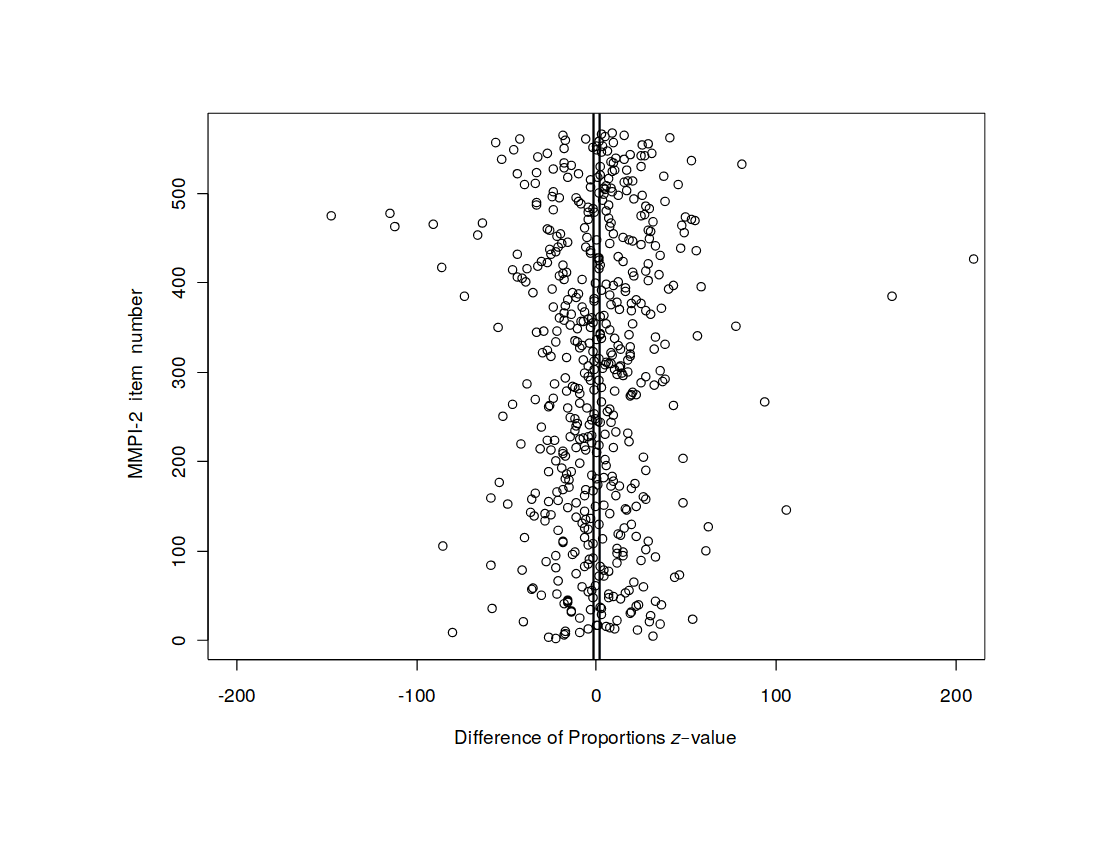
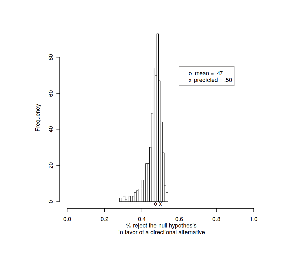


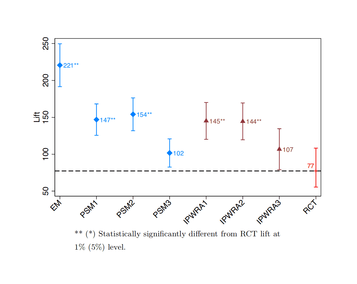
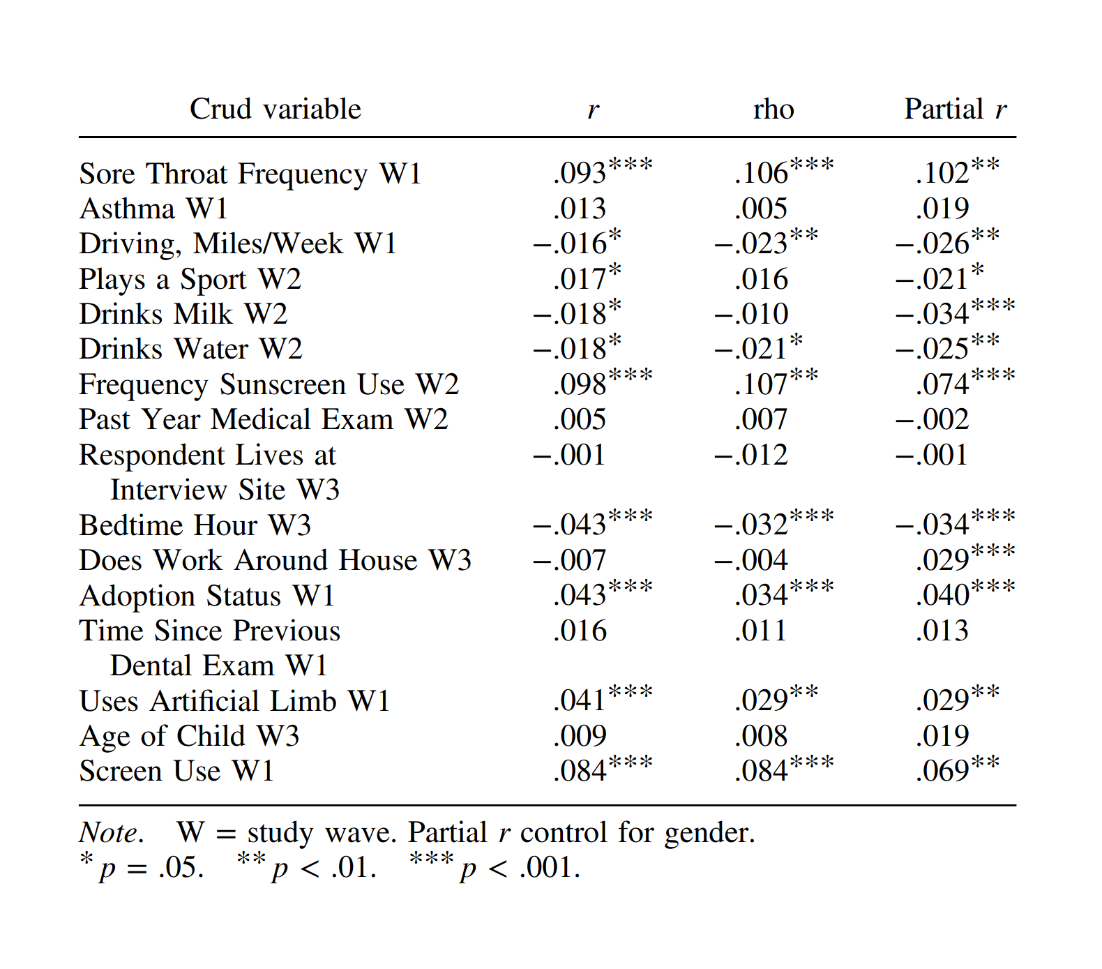
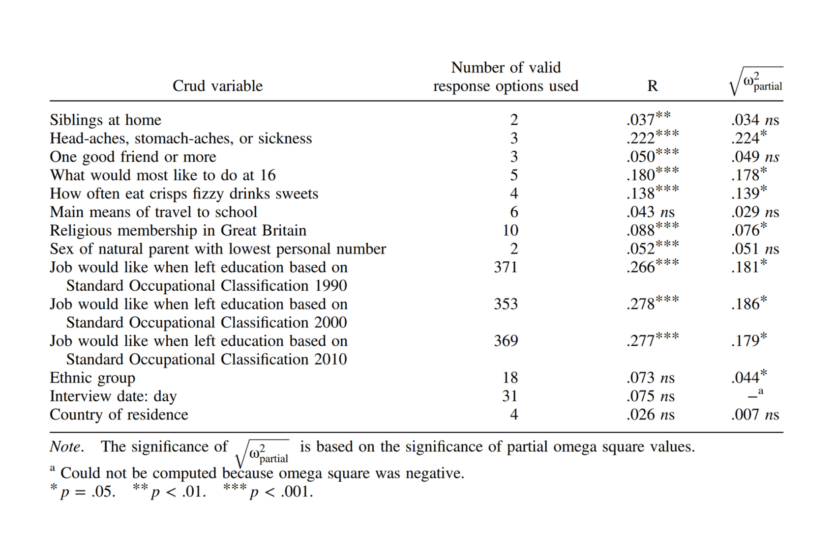
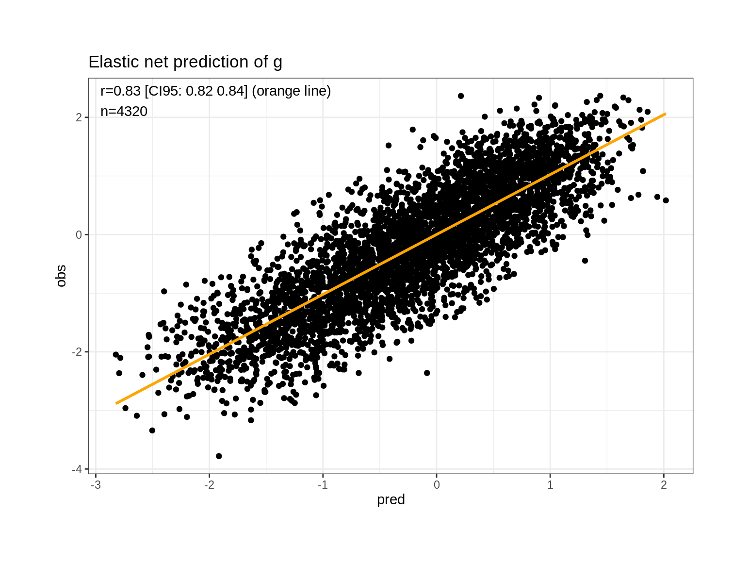
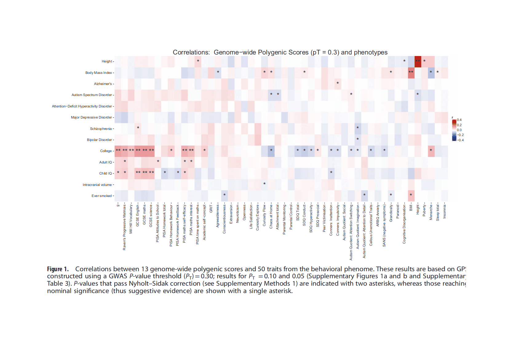
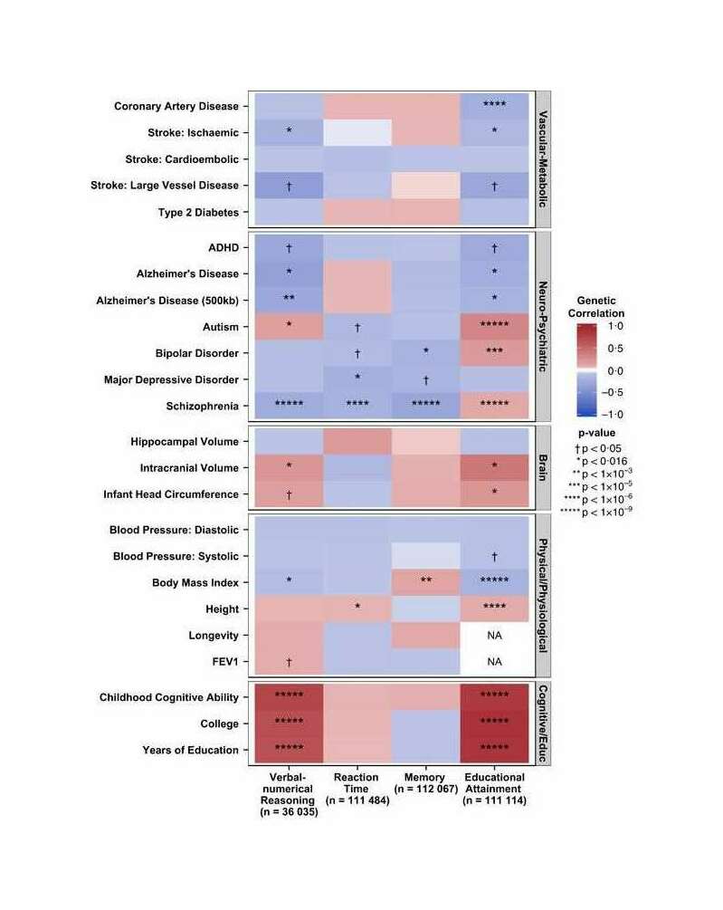
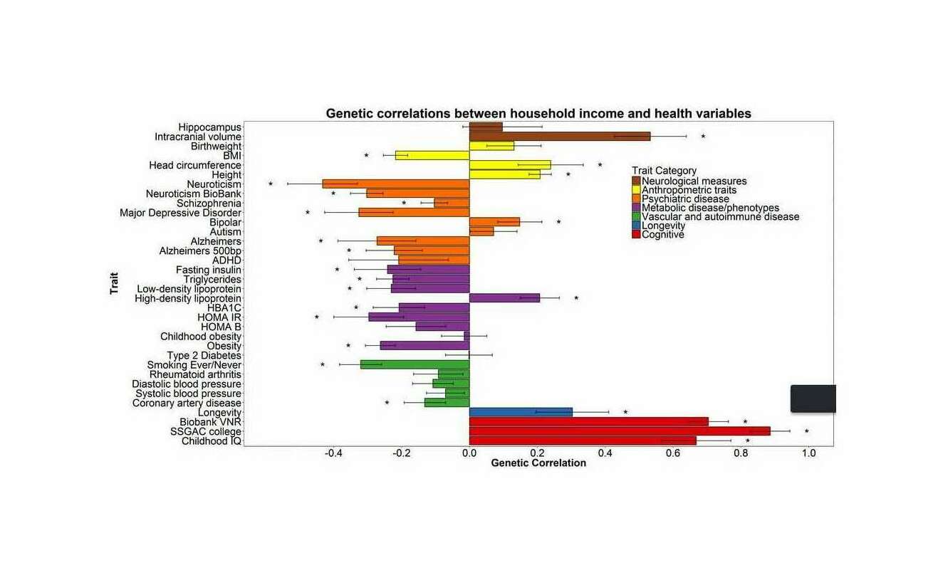
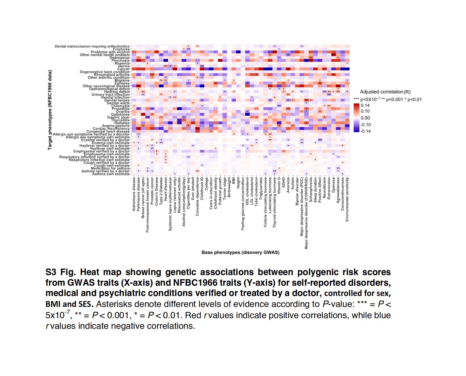
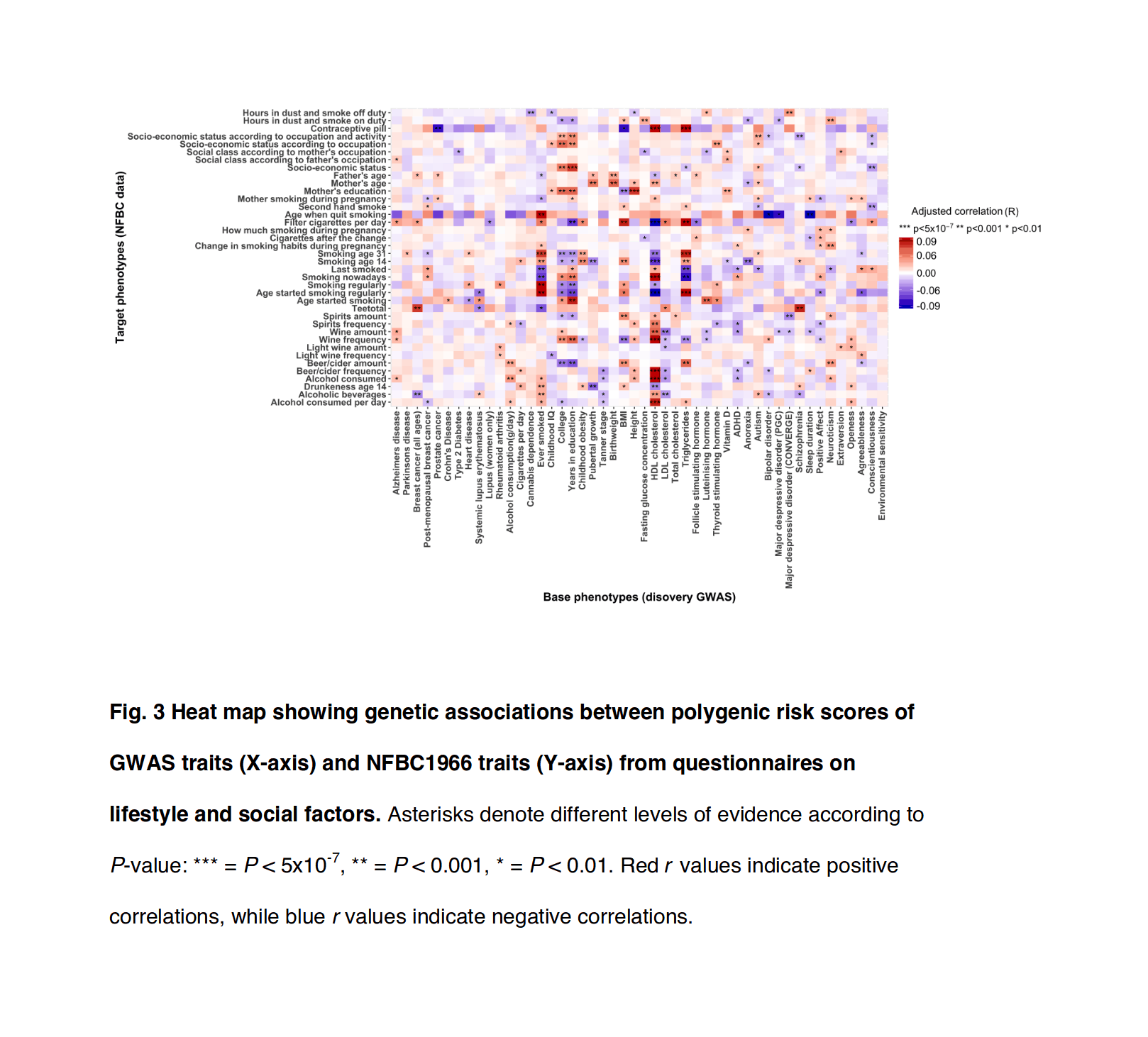
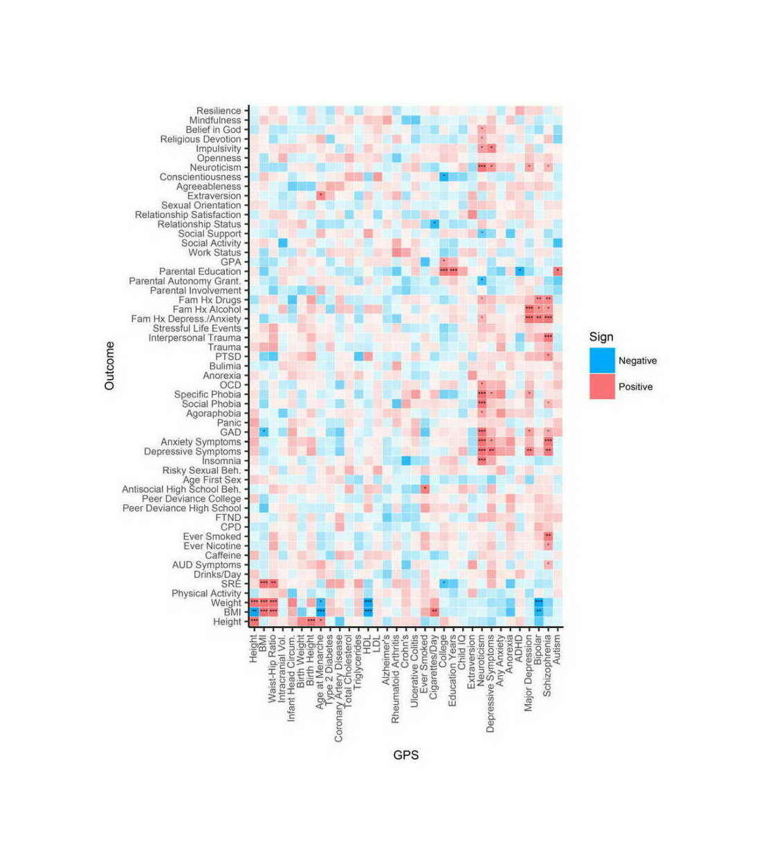
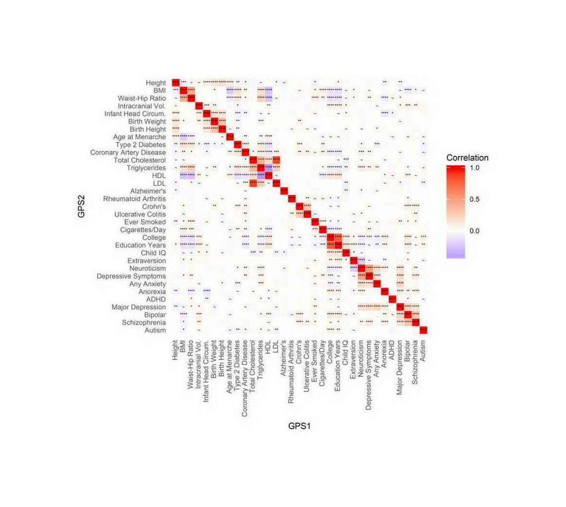
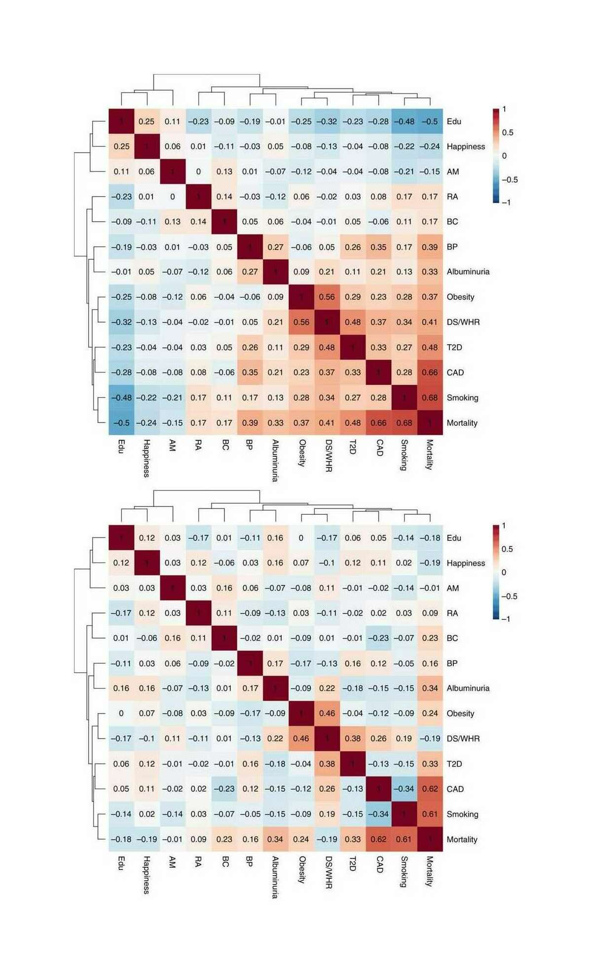
![“Fig. 4: Heat map showing the genetic correlations between the meta-analytic intelligence phenotype, intelligence, education with 29 cognitive, SES, mental health, metabolic, health and wellbeing, anthropometric, and reproductive traits. Positive genetic correlations are shown in green and negative genetic correlations are shown in red. Statistical-significance following FDR (using Benjamini-Hochberg procedure [51]) correction is indicated by an asterisk.”](/doc/genetics/heritable/correlation/2018-hill-figure5-intelligencergs.jpg)