With genetic predictors of a phenotypic trait, it is possible to select embryos during an in vitro fertilization process to increase or decrease that trait. Extending the work of Shulman & Bostrom2014/Hsu2014, I consider the case of human intelligence using SNP-based genetic prediction, finding:
a meta-analysis of GCTA results indicates that SNPs can explain >33% of variance in current intelligence scores, and >44% with better-quality phenotype testing
this sets an upper bound on the effectiveness of SNP-based selection: a gain of 9 IQ points when selecting the top embryo out of 10
the best 2016 polygenic score could achieve a gain of ~3 IQ points when selecting out of 10
the marginal cost of embryo selection (assuming IVF is already being done) is modest, at $2,076.91$1,5002016 + $276.92$2002016 per embryo, with the sequencing cost projected to drop rapidly
a model of the IVF process, incorporating number of extracted eggs, losses to abnormalities & vitrification & failed implantation & miscarriages from 2 real IVF patient populations, estimates feasible gains of 0.39 & 0.68 IQ points
embryo selection is currently unprofitable (mean: −$495.69$3582016) in the USA under the lowest estimate of the value of an IQ point, but profitable under the highest (mean: $8,626.11$6,2302016). The main constraints on selection profitability is the polygenic score; under the highest value, the NPV EVPI of a perfect SNP predictor is $33.23$242016b and the EVSI per education/SNP sample is $98.31$712016k
under the worst-case estimate, selection can be made profitable with a better polygenic score, which would require n > 237,300 using education phenotype data (and much less using fluid intelligence measures)
selection can be made more effective by selecting on multiple phenotype traits: considering an example using 7 traits (IQ/height/BMI/diabetes/ADHD/bipolar/schizophrenia), there is a factor gain over IQ alone; the outperformance of multiple selection remains after adjusting for genetic correlations & polygenic scores and using a broader set of 16 traits.
Before going into a detailed cost-benefit analysis of embryo selection, I’ll give a rough overview of the various developing approaches for genetic engineering of complex traits in humans, compare them, and briefly discuss possible timelines and outcomes. (References/analyses/code for particular claims are generally provided in the rest of the text, or in some cases, buried in my embryo editing rough notes, and omitted here for clarity.)
The past 2 decades have seen a revolution in molecular genetics: the sequencing of the human genome kicked off an exponential reduction in genetic sequencing costs which have dropped the cost of genome sequencing from millions of dollars to $27.69$202016 (SNP genotyping)–$692.3$5002016 (whole genomes). This has enabled the accumulation of datasets of millions of individuals’ genomes which allow a range of genetic analyses to be conducted, ranging from SNP heritabilities to detection of recent evolution to GWASes of traits to estimation of the genetic overlap of traits.
The simple summary of the results to date is: behavioral genetics was right. Almost all human traits, simple and complex, are caused by a joint combination of environment, stochastic & randomness, and genes. These patterns can be studied by methods such as family, twin, adoption, or sibling studies, but ideally are studied directly by reading the genes of hundreds of thousands of unrelated people, which yield estimates of the effects of specific genes and predictions of phenotype values from entire genomes. Across all traits examined, genes cause ~50% of differences between people in the same environment, factors like randomness & measurement-error explain much of the rest, and whatever is left over is the effect of nurture. Evolution is true, and genes are discrete physical patterns encoded in chromosomes which can be read and edited, with simple traits such as many diseases being determined by a handful of genes, yielding complicated but discrete behavior, while complex traits are instead governed by hundreds or thousands of genes whose effects sum together and produce a normal distribution such as IQ or risk of developing a complicated disease like schizophrenia. This allows direct estimation of their genetic contribution to a phenotype, as well as that of their children. These genetic traits contribute to many observed societal patterns, such as the children of the rich also being richer and smarter and healthier, why poorer neighborhoods have sicker people, relatives of schizophrenics are less intelligent, etc.; these traits are substantially heritable, and traits are also interconnected in an intricate web of correlations where one trait causes another and both are caused by the same genetic variants. For example, intelligence-related variants are uniformly inversely correlated with disease-related variants, and positively correlated with desirable traits. These results have been validated by many different approaches and the existence of widespread large heritabilities, genetic correlations, and valid PGSes are now academic consensus.
Because of this pervasive genetic influence on outcomes, genetic engineering is one of the great open questions in transhumanism: how much is possible, with what, and when?
Suggested interventions can be broken down into a few categories:
cloning (copying)
selection (variation with ranking)
editing (rewriting)
synthesis (writing)
Each of these has different potentials, costs, and advantages & disadvantages:
An opinionated comparison of possible interventions, focusing on potential for improvements, power, and cost.
Intervention
Description
Time
Cost
Limits
Advantages
Disadvantages
Cloning
Somatic cells are harvested from a human and their DNA transferred into an embryo, replacing the original DNA. The embryo is implanted. The result is equivalent to an identical twin of the donor, and if the donor is selected for high trait-values, will also have high trait-values but will regress to the mean depending on the heritability of said traits.
?
$100k?
cannot exceed trait-values of donor, limited by best donor availability
does not require any knowledge of PGSes or causal variants, is likely doable relatively soon as modest extension of existing mammalian cloning, immediate gains of 3-4SD (maximum possible global donor after regression to mean)
may trigger taboos & is illegal in many jurisdictions, human cloning has been minimally researched, hard to find parents as clone will be genetically related to one parent at most & possibly neither, can’t be used to get rare or new genetic variants, inherently limited to regressed maximum selected donor, does not scale in any way with more inputs
Simple (Single-Trait) Embryo Selection
A few eggs are extracted from a woman and fertilized; each resulting sibling embryo is biopsied for a few cells which are sequenced. A single polygenic score is used to rank the embryos by predicted future trait-value, and surviving embryos are implanted one by one until a healthy live birth happens or there are no more embryos. By starting with the top-ranked embryo, an average gain is realized.
0 years
$1k-$5k
egg count, IVF yield, PGS power
offspring fully related to parents, doable & profitable now, doesn’t require knowledge of causal variants, doesn’t risk off-target mutations, inherently safe gains, PGSes steadily improving
permanently limited to <1SD increases on trait, requires IVF so I am doubtful it’ could ever exceed ~10% US population usage, fails to benefit from using good genetic correlations to boost overlapping traits & avoid harm from negative correlations (where a good thing increases a bad thing), biopsy-sequencing imposes fixed per-embryo costs, fast diminishing returns to improvements, can only select on relatively common variants currently well-estimated by PGSes & cannot do anything about fixed variants neither or both parents carry
Simple Multiple (Trait) Embryo Selection
*, but the PGS used for ranking is a weighted sum of multiple (possibly scores or hundreds) of PGSes of individual traits, weighted by utility.
*
*
*
*, but several times larger gains from selection on multiple traits
*, but avoids harms from bad genetic correlations
Massive Multiple Embryo Selection
A set of eggs is extracted from a woman, or alternately, some somatic cells like skin cells. If immature eggs in an ovary biopsy, they are matured in vitro to eggs; if somatic cells, they are regressed to stem cells, possibly replicated hundreds of times, and then turned into egg-generating-cells and finally eggs, yielding hundreds or thousands of eggs (all still identical to her own eggs). Either way, the resulting large number of eggs are then fertilized (up to a few hundred will likely be economically optimal), and then selection & implantation proceeds are as in simple multiple embryo selection.
>5 years
$5k->$100k
sequencing+biopsy fixed costs, PGS power
offspring fully related to parents, lifts main binding limitation on simple multiple embryo selection, allowing potentially 1-5SD gains depending on budget, highly likely to be at least theoretically possible in next decade
cost of biopsy+sequencing scales linearly with number of embryos while encountering further diminishing returns than experienced in simple multiple embryo selection, may be difficult to prove new eggs are as long-term healthy
Donor sperm and eggs are (somehow) sequenced; the ones with the highest-ranked chromosomes are selected to fertilize each other; this can then be combined with simple or massive embryo selection. It may be possible to fuse or split chromosomes for more variance & thus selection gains.
? years
$1?-$5k?
ability to non-destructively sequence or infer PGSes of gametes rather than embryos, PGS power
immediate large boost of ~2SD possible by selecting earlier in the process before variance has been canceled out, does not require any new technology other than the gamete sequencing part
how do you sequence sperm/eggs non-destructively?
Iterated embryo selection (IES)
(Also called “whizzogenetics”, “in vitro eugenics”, or “in vitro breeding”/IVB.) A large set of cells, perhaps from a diverse set of donors, is regressed to stem cells, turned into both sperm/egg cells, fertilizing each other, and then the top-ranked embryos are selected, yielding a moderate gain; those embryos are not implanted but regressed back to stem cells, and the cycle repeats. Each “generation” the increases accumulate; after perhaps a dozen generations, the trait-values have increased many SDs, and the final embryos are then implanted.
>10 years
$1m?-$100m?
full gametogenesis control, total budget, PGS power
can attain maximum total possible gains, lessened IVF requirement (implantation but not the egg extraction), current PGSes adequate
full & reliable control of gamete⟺stem-cell⟺embryo pipeline difficult & requires fundamental biology breakthroughs, running multiple generations may be extremely expensive and gains limited in practice, still restricted to common variants & variants present in original donors, unclear effects of going many SDs up in trait-values, so expensive that embryos may have to be unrelated to future parents as IES cannot be done custom for every pair of prospective parents, may not be feasible for decades
A set of embryos are injected with gene editing agents (eg. CRISPR delivered via viruses or micro-pellets), which directly modify DNA base-pairs in some desired fashion. The embryos are then implanted. Similar approaches might be to instead try to edit the mother’s ovaries or the father’s testicles using a viral agent.
0 years
<$10k
offspring fully related to parents, causal variant problem, number of safe edits, edit error rate
gains independent of embryo number (assuming no deep sequencing to check for mutations), potentially arbitrarily cheap, potentially unbounded gains doesn’t require biopsy-sequencing, unknown upper bound on how many possible total edits, can add rare or unique genes
each edit adds little, edits inherently risky and may damage cells through off-target mutations or the delivery mechanism itself, requires identification of the generally-unknown causal genes rather than predictive ones from PGSes, currently doesn’t scale to more than a few (unique) edits, most approaches would require IVF, parental editing inherently halves the possible gain
Genome Synthesis
Chemical reactions are used to build up a strand of custom DNA literally base-pair by base-pair, which then becomes a chromosome. This process can be repeated for each chromosome necessary for a human cell. Once one or more of the chromosomes are synthesized, they can replace the original chromosomes in a human cell. The synthesized DNA can be anything, so it can be based on a polygenic score in which every SNP or genetic variant is set to the estimated best version.
>10 years (single chromosomes) to >15 years whole genome?
$30m-$1b
cost per base-pair, overall reliability of synthesis
achieves maximum total possible gains across all possible traits, is not limited to common variants & can implement any desired change, cost scales with genome replacement percentage (with an upper bound at replacing the whole genome), cost per base-pair falling exponentially for decades and HGP-Rewrite may accelerate cost decrease, many possible approaches for genome synthesis & countless valuable research or commercial applications driving development, current PGSes adequate
full genome synthesis would cost ~$1b, error rate in synthesized genomes may be unacceptably high, embryos may be unrelated to parents due to cost like IES, likely not feasible for decades
Overall I would summarize the state of the field as:
cloning: is unlikely to be used at any scale for the foreseeable future despite its power, and so can be ignored (except inasmuch as it might be useful in another technology like IES or genome synthesis)
simple single-trait embryo selection: is strictly inferior to simple multiple embryo selection, and there is no reason to use it other than the desire to save a tiny bit of statistical effort, and much reason to use multiple-trait selection instead (larger and safer gains), so single-trait selection need not be discussed except as a strawman or pedagogical example.
simple multiple-trait embryo selection: available & profitable now (first baby was born mid-2020), but is too limited in possible gains, requires a far too onerous process (IVF) for more than a small percentage of the population to use it, and is more or less trivial in consequences.
As median embryo count in IVF hovers around 5, the total gain from selection is small, and much of the gain is wasted by losses in the IVF process (the best embryo doesn’t survive storage, the second-best fails to implant, and so on). One of the key problems is that polygenic scores are the sum of many individual small genes’ effects and form a normal distribution, which is tightly clustered around a mean. A polygenic score is attempting to predict the net effect of thousands of genes which almost all cancel out, so even accurate identification of many relevant genes still yields an apparently unimpressive predictive power. The fact that traits are normally distributed also creates difficulties for selection: the further into the tail one wants to go, the larger the sample required to reach the next step—to put it another way, if you have 10 samples, it’s easy (a 1 in 10 probability) that your next random sample will be the largest sample yet, but if you have 100 samples, now the probability of an improvement is the much harder 1 in 100, and if you have 1,000, it’s only 1 in 1,000; and worse, if you luck out and there’s an improvement, the improvement is ever tinier. After taking into account existing PGSes, previously reported IVF process losses, costs, and so on, the implication that it is moderately profitable and can increase traits perhaps 0.1SD, rising somewhat over the next decade as PGSes continue to improve, but never exceeding, say, 0.5SD.
Embryo selection could have substantial societal impacts in the long run, especially over multiple generations, but this would both require IVF to become more common and for no other technology to supersede it (as they certainly shall). When IVF began, many pundits proclaimed it would “forever change what it means to be human” and other similar fatuosities; it did no such thing, and has since productively helped countless parents & children, and I fully expect embryo selection to go the same way. I would consider embryo selection to have been considerably overhyped (by those hyperventilating about “Gattaca being around the corner”), and, ironically, also underhyped (by those making arguments like “trait X is so polygenic, therefore embryo selection can’t work”, which is statistically illiterate, or “traits are complex interactions between genes and environment most of which we will never understand”, which is obfuscating irrelevancy and FUD).
Embryo selection does have the advantage of being the easiest to analyze & discuss, and the most immediately relevant.
massive multiple embryo selection: the single most binding constraint on simple embryo selection (single or multiple trait), is the number of embryos to work with, which, since paternal sperm is effectively infinite, means number of eggs.
For selection, the key question is what is the most extreme or maximum item in the sample; a small sample will not spread wide, but a large sample will have a bigger extreme. The more lottery tickets you buy, the better the chance of getting 1 ticket which wins a lot. Whereas, the PGS, to peoples’ general surprise, doesn’t make all that much of a difference after a little while. If you have 3 embryos, even going from a noisy to a perfect predictor, it doesn’t make much of a difference, because no matter how flawless your prediction, embryo #1 (whichever it is) out of 3 just isn’t going to be all that much better than average; if you have 300 embryos, then a perfect predictor becomes more useful.
There is no foreseeable way to safely extract more eggs from a donor: standard IVF cycle approaches appear to have largely reached their limit, and stimulating more eggs’ release in a harvesting cycle is dangerous. A different approach is required, and it seems the only option may be to make more eggs. One possibility is to not try to stimulate release of a few eggs and collect them, but instead biopsy samples of proto-eggs and then hurry them in vitro to maturity as full eggs, and get many eggs that way; biopsies might be compelling without selection at all: the painful, protracted, failure-prone, and expensive egg harvesting process to get ~5 embryos, which then might yield a failed cycle anyway, could be replaced by a single quick biopsy under anesthesia yielding hundreds of embryos effectively ensuring a successful cycle. Less invasively, laboratory results in inducing regression to stem cell states and then oogenesis have made steady progress over the past decades in primarily rat/mice but also human cells, and researchers have begun to speak of the possibility in another 5 or 10 years of enabling infertile or homosexual couples to conceive fully genetically-related children through somatic ↔︎ gametic cell conversions. This would also likely allow generating scores or hundreds of embryos by turning easier-to-acquire cells like skin cells or extracted eggs into stem cells which can replicate and then be converted into egg cells & fertilized. While it is still fighting the normal distribution with brute force, having 500 embryos works a lot better than having just 5 embryos to choose from. The downside is that one still needs to biopsy and sequence each embryo in order to compute their particular PGS; since one is still fighting the thin tail, at some point the cost of creating & testing another embryo exceeds the expected gain (probably somewhere in the hundreds of embryos).
Unlike simple embryo selection, this could yield immediately important gains like +2SD. IVF yield ceases to be much of a problem (the second/third/fourth-best embryos are now almost exactly as good as the first-best was and they probably won’t all fail), and enough brute force has been applied to reach potentially 1-2SD in practice. If taken up by only the current IVF users and applied to intelligence alone, it would immediately lead to the next generation’s elite positions being dominated by their kids; if taken up by more and done properly on multiple traits, the advantage would be greater.
Gamete selection/Optimal Chromosome Selection: only a theoretical possibility at the moment, as there is no direct way to sequence individual sperm/eggs or manipulate chromosome choice. GS/OCS are interesting more for the points they make about variance & order statistics & the CLT: it results in a much larger gain than one would expect simply by switching perspectives and focusing on how to select earlier in the ‘pipeline’, so to speak, where variance is greater because sets of genes haven’t yet been combined in one package & canceled each other out. If someone did something clever to allow inference on gametes’ PGSes or select individual chromosomes, then it could yield an immediate discontinuously large boost in trait-value of +2SD in conjunction with whatever embryo selection is available at that point.
Iterated Embryo Selection: If IES were to happen, it would allow for almost arbitrarily large increases in trait-values across the board in a short period of time, perhaps a year. While IES has major disadvantages (extremely costly to produce the first optimized embryos, depending on how many generations of selection are involved; selection has some inherent speed limits trading off between accidentally losing possibly useful variants & getting as large a gain each generation as possible; embryos are unlikely to resemble the original donors at all without an additional generation ‘backcrossed’ with the original donor cells, undoing most of the work), the extreme increases may justify use of IES and create demand from parents. This could then start a tsunami. Depending on how far IES is pushed, the first release of IES-optimized embryos may become one of the most important events in human history.
IES is still distant and depends on a large number of wet lab breakthroughs and finetuned human-cell protocols. Coaxing scores or hundred of cells through all the stages of development and fertilization, for multiple generations, is no easy task. When will IES be possible? The relevant literature is highly technical and only an expert can make sense of it, and one should have hands-on expertise to even try to make forecasts. There are no clear cost curves or laws governing progress in stem cell/gamete research which can be used to extrapolate. Perhaps no one will ever put all the money and consistent research effort into developing it into something which could be used clinically. Just because something is theoretically possible and has lots of lab prototypes doesn’t mean that the transition will happen. (Look at human cloning; everyone assumed it’d happen long ago, but as far as anyone knows, it never has.) On the other hand, perhaps someone will.
IES is one of the scariest possibilities on the list, and the hardest to evaluate; it seems clear, at least, that it will certainly not happen in the next decade, but after that…? IES has been badly under-discussed to date.
Gene Editing: the development of CRISPR has led to more hype than embryo selection itself. However, the current family of CRISPR techniques & previous alternatives & future improvements, can be largely dismissed on statistical grounds alone. Even if we hypothesized some super-CRISPR which could make a handful of arbitrary SNP edits with zero risk of mutation or other forms of harm, it would not be especially useful and would struggle to be competitive with embryo selection, let alone IES/OCS/genome synthesis. The unfixable root cause is the polygenicity of the most important polygenic traits (which is a blessing for selection or synthesis approaches, as it creates a vast reservoir of potential improvements, but a curse for editing), and to a lesser extent, the asymmetry of effect sizes (harmful variants are more harmful than beneficial ones are beneficial).
The benefit of gene editing a SNP is the number of edits times the SNP effect of each edit times the probability the effect is causal. Probability it’s causal? Can’t we assume that the top hits from large GWASes these days have a posterior probability ~100% of having a non-zero effect? No. This is because of a technical detail which is largely irrelevant to selection processes but is vitally important to editing: the hits identified in a PGS are not necessarily the exact causal base-pair(s). Often they are, but more often they are not. They are instead proxies for a neighboring causal variant which happens to usually be inherited with it, as genomes are inherited in a chunky fashion, in big blocks, and do not split & recombine at every single base-pair. This is no problem for selection—it predicts great and is cheaper & easier to find a correlated SNP than the true causal variant. But it is fatal to editing: if you edit a proxy, it’ll do nothing (or maybe it’ll do the opposite).
How fatal is this? Attempts at “fine-mapping” or using large datasets to distinguish which of a few SNPs is the real culprit or seeing how PGSes’ performance shrinks when going from the original GWAS population to a deeply genetically different population like Subsaharan Africans who have totally different proxy patterns (if there is non-zero prediction power, it must be thanks to the causal hits, which act the same way in both populations), we can estimate that the causal probability may be as low as 10%. Combine this with the few edits safely permitted, perhaps 5, the small effect size of each genetic variant, like 0.2 IQ points for intelligence, and the effect becomes dismal. A tenth of a point? Not much. Even if we had all causal variants, the small average effect size, combined with few possible edits, is no good. Fix the causal variant problem, and it’s still only 5 edits at 0.2 points each. Nor is IQ at all unique in this respect—it’s somewhat unusually polygenic, but a cleaner trait like height still implies small gains such as half an inch.
What about rare variants? The problem with rare variants is that they are rare, and also not of especially large beneficial effect. Being rare makes them hard to find in the first place, and the lack of benefit (as compared to a baseline human without said variant) means that they are not useful for editing. We might find many variants which damage a trait by a large amount, say, increasing abdominal fat mass by a kilogram or lowering IQ by a dozen points, but of course, we don’t want to edit those in! (They also aren’t that important for any embryo selection method, because they are rare, not usually present, and thus there is usually no selection to be done.) We could hope to find some variant which increases IQ by several points—but none have been found, if they were at all common they would’ve been found a long time ago, and indirect methods like DeFries-Fulker regression suggest that there are few or no such rare variants. Nor is measuring other traits a panacea: if there were some variant which increased IQ by a medium amount by increasing a specific trait like working memory which has not been studied in large GWASes or DeFries-Fulker regressions to date, then such a WM-boosting variant should’ve been detected through its mediated effect, and to the extent that it has no effect on hard endpoints like IQ or education or income, it then must be questioned how useful it is in the first place. The situation may be somewhat better with other traits (there’s still hope for finding large beneficial effects1, and in the other direction, disease traits tend to have more rare variants of larger effects which might be worth fixing in relatively many individual cases, like BRCA or APOE) but I just don’t see any realistic way to reach gains like +1SD on anything with gene editing methods in the foreseeable future using existing variants.
What about non-existing variants ie brand-new variants based on extrapolation from human genetic history or animal models? These hypothetical mutations/edits could have large effects even if we have failed to find any in the wild. But the track record of animal models in predicting complex human systems such as the brain is not good at all, and such large novel mutations would have zero safety record, and how would you prove any were safe without dozens of live births and long-term followup—which would never be permitted? Given the poor prior probability of both safety & efficacy, such mutations would simply remain untried indefinitely.
It is difficult to see how to remedy this in any useful way. The causal probability will creep up as datasets expand & cross-racial GWASes become more common, but that doesn’t resolve the issue after we increase the gain by a factor of 10. The limit is still the edit count: the unique edit limit of ~5 is not enough to work with. Can this be combined usefully with IES to do edits per generation? Likely but you still need IES first! Can the edit limit be lifted? …Maybe. Genetic editing follows no predictable improvement curve, or learning curve, and doesn’t benefit directly from any exponentials. It is hard to forecast what improvements may happen. 2019 saw a breakthrough from a repeated-edit SOTA of ~60 edits in a cell to ~2,600 (Smith et al 2019), which no one forecast, but it’s unclear when if ever that would transfer to useful per-SNP edits; but nevertheless, the possibility of mass editing cannot be ruled out.
So, CRISPR-style editing may be revolutionary in rare genetic diseases, agriculture, & research, but as far as we are concerned, it has been grossly overhyped: there is a chance it will live up to the most extreme claims, but not a large one.
Genome synthesis: the simple answer to gene editing’s failure is to observe that if you have to make possibly thousands of edits to fix up a genome to the level you want it, why not go out and make your own genome? (with blackjack and hookers…) That is the audacious proposal of genome synthesis. It sounds crazy, since genome synthesis has historically been mostly used to make short segments for research, or perhaps the odd pandemic virus, but unnoticed by most, the cost per base-pair has been crashing for decades, allowing the creation of entire yeast genomes and leading to the recent HGP-Write proposal from George Church & others to invest in genome synthesis research with the aim of inventing methods which can create custom genomes at reasonable prices. Such an ability would be staggeringly useful: custom organisms designed to produce arbitrary substances, genomes with the fundamental encoding all swapped around rendering them immune to all viruses ever, organisms with a single giant genome or with all mutations replaced with the modal gene, among other crazy things. One could also, incidentally, use cheap genome synthesis for bulk storage of data in a dense, durable, room-temperature format (explaining both Microsoft & IARPA’s interest in funding genome synthesis research).
Of course, if you can synthesize an entire genome—a single chromosome would be almost as good to some extent—you can take a baseline genome and make as many ‘edits’ as you please. Set all the top variants for all the relevant traits to the estimated best setting. The possible gains are greater than IES (since you are not limited by the initial gene pool of starting variants nor by the selection process itself), and one can increase traits by hundreds of SDs (whatever that means).
Genome synthesis, unlike IES, has historically proceeded on a smooth cost-curve, has many possible implementations, and has many research groups & startups involved due to its commercial applications. A large-scale “HGP-Write” has been proposed to scale genome synthesis up to yeast sized organisms and eventually human-sized genomes. The cost curve suggests that around 2035, whole human genomes reach well-resourced research project ranges of $10-30m; some individuals in genome synthesis tell me they are optimistic that new methods can greatly accelerate the cost-curve. (Unlike IES, genome synthesis is not committed to a particular workflow, but can use any method which yields, in the end, the desired genome; all of these methods can be researched in parallel & only one needs to work, representing a major advantage.) Genome synthesis has many challenges before one could realistically implant an embryo, such as ensuring all the relevant structural features like methylation are correct (which may not have been necessary for earlier more primitive/robust organisms like yeast), and so on, but whatever the challenges for genome synthesis, the ones for IES appear greater. It is entirely possible that IES will develop too slowly and will be obsoleted by genome synthesis in 10-20 years. The consequences of genome synthesis would be, if anything, larger than IES because the synthesis technology will be distributed in bulk, will probably continue decreasing in cost due to the commercial applications regardless of human use, and don’t require rare specialized wet lab expertise but like genome sequencing, will almost certainly become highly automated & ‘push button’.
If IES has been under-discussed and is underrated, genome synthesis has not been discussed at all & vastly more underrated.
To sum up the timeline: CRISPR & cloning are already available but will remain unimportant indefinitely for various fundamental reasons; multiple embryo selection is useful now but will always be minor; massive multiple embryo selection is some ways off but increasingly inevitable and the gains are large enough on both individual & societal levels to result in a shock; IES will come sometime after massive multiple embryo selection but it’s impossible to say when, although the consequences are potentially global; genome synthesis is a similar level of seriousness, but is much more predictable and can be looked for, very loosely, 2030–102040 (and possibly sooner).
Readers already familiar with the idea of embryo selection may have some common misconceptions which would be good to address up front:
IVF Costs: IVF is expensive, somewhat dangerous, and may have worse health outcomes than natural childbirth
I agree, but we can consider the case where these issues are irrelevant. It is unclear what the long-run effects of IVF on children may be, other than the harm probably isn’t too great; the literature on IVF suggests that the harms are probably very small and smaller than, for example, paternal age effects, but it’s hard to be sure given that IVF usage is hardly exogenous and good comparison groups for even just correlational analysis are hard to come by. (Natural-born children are clearly not comparable, but neither are natural-born siblings of IVF children—why was their mother able to have one child naturally but needed IVF for the next?) I would not recommend anyone do IVF solely to benefit from embryo selection (as opposed to doing PGD to avoid passing a horrible genetic disease like Huntington’s, where it is impossible for the hypothetical harms of IVF to outweigh the very real harm of that genetic disease). Here I consider the case where parents are already doing IVF, for whatever reason, and so the potential harms are a “sunk cost”: they will happen regardless of the choice to do embryo selection, and can be ignored. This restricts any results to that small subset (~1% of parents in the USA as of 2016), of course, but that subset is the most relevant one at present, is going to grow over time, and could still have important societal effects.
An interesting question would be, at what point does embryo selection become so compelling that would-be parents with a family history of disease (such as schizophrenia) would want to do it? (Because of the nonlinear nature of liability-threshold polygenic traits and relatively rare diseases like schizophrenia, someone with a family history benefits far more than someone with an average risk; see the truncation selection/multiple-trait selection on why this implies that selection against diseases is not as useful as it seems.) What about would-be parents with no particular history? How good does embryo selection need to be for would-be parents who could conceive naturally to be willing to undergo the cost (~$10k even at the cheapest fertility clinics) and health risks (for both mother & child) to benefit from embryo selection? I don’t know, but I suspect “simple embryo selection” is too weak and it will require “massive embryo selection” (see the overview for definitions & comparisons).
PGSes Don’t Work: GWASes merely produce false positives and can’t do anything useful for embryo selection because they are false positives/population structure/publication bias/etc…
Some readers overgeneralize the debacle of the candidate-gene literature, which is almost 100% false-positive garbage, to GWASes; but GWASes were designed in response to the failure of candidate-genes by much more stringent thresholds & large datasets & more population structure correction, and have performed well as datasets reached necessary sizes. Their PGSes predict out-of-sample increasingly large amounts of variance, the PGSes have high genetic correlations between cohorts/countries/times/measurement methods, and they work within-family between siblings, who by definition have identical ancestries/family backgrounds/SES/etc but have randomized inheritance from their parents. For a more detailed discussion, see the section, “Why Trust GWASes?”. (While GWASes are indeed highly flawed, those flaws typically work in the direction of inefficiency/reducing their predictive power, not inflating them.)
The Prediction Is Noncausal: GWASes may be predictive but this is irrelevant because the SNPs in a PGS are merely non-causal variants which proxy for causal variants
Background: in a GWAS, the measured SNPs may cause the outcome or they may merely be located on a genome nearby a genetic variant which has the causal effect; because genomes are inherited in a ‘chunky’ fashion, a measured SNP may almost always be found alongside the causal genetic variant within a particular population. (Over a long enough timeframe, as organisms reproduce, that part of the genome will be broken up, but this may take centuries or millennia.) Such a SNP is in “linkage disequilibrium” or just LD. Such a scenario is quite common, and may in fact be the case for the overwhelming majority of SNPs in human GWASes. This is both a blessing and a curse for GWASes: it means that easy cheaply-measured SNPs can probe harder-to-find genetic variants, but it also means that the SNPs are not causal themselves. So for example, if one took a list of SNPs from a GWAS, and used CRISPR to edit them, most of the edits would do nothing. This is a serious concern for genetic engineering approaches—just because you have a successful GWAS doesn’t mean you know what to edit!
But is this a problem for embryo selection? No. Because you are not engaged in any editing or causal manipulation. You are passively observing and predicting what is the best embryo in a sample. This does not disturb the LD patterns or break any correlations, and the predictions remain valid. Selection doesn’t care what the causal variants are, it cares only that, whatever they are or wherever they are on the genome, the chosen embryo has more of them than the not-chosen embryos. Any proxy will do, as long as it predicts well. In the long run, changes in LD will gradually reduce the PGS’s predictive power as the SNPs become better/worse proxies, but this is unimportant since there will be many GWASes in between now and then, and one would be upgrading PGSes for other reasons (like their steadily improving predictive power regardless of LD patterns).
PGSes Predict Too Little: Embryo selection can’t be useful with PGSes predicting only X% [where X% > state-of-the-art] of individual variance
The mistake here is confusing a statistical measure of error with the goal. Any default summary statistic like R2 or RMSE is merely a crutch with tenuous connections to optimal decisions. In embryo selection, the goal is to choose better embryos than average to implant rather than implant random embryos, to get a gain which pays for the costs involved. A PGS only needs to be accurate enough to select a better embryo out of a (typically small) batch. It doesn’t need to be able to predict future, say, IQ, within a point. Estimating the precise future trait value of an embryo may be quite difficult, but it’s much easier to predict which of two embryos will have a higher trait value. (It’s the difference between predicting the winner of a soccer game and predicting the exact final score; the latter does let one do the former, but the former is what one needs and is much easier.) Once your PGS is good enough to pick the best or near-best embryo, even a far better PGS makes little difference—after all, one can’t do any better than picking the best embryo out of a batch. And due to diminishing returns/tail effects, the larger the batch, the smaller the difference between the best and the 4th-best etc., reducing the regret. (In a batch of 2, there’s little difference between a poor and a perfect predictor; and in a batch of 1, there’s none.)
To decide whether a PGS of X% is adequate cannot be done in a vacuum; the necessary performance will depend critically on the value of a trait, the cost of embryo selection, the losses in the IVF pipeline, and most importantly of all, the number of embryos in each batch. (The final gain depends the most on the embryo count—a fact lost on most people discussing this topic.) As embryo selection is cheap at the margin, and ranking is easier than regression, this can be done with surprisingly poor PGSes, and the bar of profitability is easy to meet, and for embryo selection, has been met for some years now (see the rest of this page for an analysis of the specific case of IQ).
Statistical-significance thresholds are essentially arbitrary. There is no need to fetishize them: they do not correspond to any posterior probability of a hit being “real”, introduce many serious difficulties of interpretation due to power (if a GWAS has a hit on an SNP with an estimated effect size of X, and a second GWAS also estimates it at X but due to a slightly higher standard error, it is no longer “statistically-significant”, what does that mean, exactly?) and even if they did, the number of false positives has little relationship to the predictive power, much less selection gain of a PGS, much less the final profit of embryo selection. The relevant question is what are the best predictions which can be made? For human complex traits, the most accurate predictions typically use a PGS based on most of or all measured variants. Anything less is less.
Unintended Consequences: Selection on traits, especially intelligence, will backfire horribly
It is hypothetically possible for selection on one trait, which happens to be inversely correlated on a genetic level, with another important trait, to backfire by increasing the first trait but then doing much more damage by decreasing the second trait. This occurs occasionally in long-term or intense breeding programs, and has been demonstrated by very carefully-designed group-selection experiments such as the famous chicken-crate experiment.
However, for humans, such genetic correlations are highly unlikely a priori as we can simply observe broad patterns like the global correlations of SES/wealth/intelligence/health with all desirable outcomes (“Cheverud’s conjecture”), and countless human genetic correlations have already been calculated by various methods and are now routinely reported in GWASes, and invariably diseases positively correlate with diseases and good things correlate with other good things. Whatever harmful backfire effects there may be are far outweighed by the beneficial backfire effects, so selection on a single trait, especially intelligence, is not going to incur these speculative hypothetical harms.
If there are any such harms, they can be reduced or eliminated by simply taking into account multiple traits while selecting, and doing multi-trait selection. This is easy to do with the present availability of PGSes on hundreds of traits—given that all the hard work is in the genotyping step, why would one ignore all traits but one and throw away all that data? In fact, even if there were no possibility of backfire effects, embryo selection would be done with multi-trait selection anyway, simply because it is so easy and the benefits are so compelling: using multiple traits allows for much greater overall gains because two embryos similar or identical on one trait may differ a great deal on another trait, and when traits are genetically correlated, they can serve as proxies for each other, producing effective boosts in predictive power. For all these reasons, most breeding programs use multi-trait selection. For more details and an example of the benefits in embryo selection, see the multiple-selection section.
Forty years ago, I could say in the Whole Earth Catalog, ‘we are as gods, we might as well get good at it’…What I’m saying now is we are as gods and have to get good at it.
In vitro fertilization (IVF) is a medical procedure for infertile women in which eggs are extracted, fertilized with sperm, allowed to develop into an embryo, and the embryo injected into their womb to induce pregnancy. The choice of embryo to implant is usually arbitrary, with some simple screening for gross abnormalities like missing chromosomes or other cellular defects, which would either be fatal to the embryo’s development (so useless & wasteful to implant) or cause birth defects like Down syndrome (so much preferable to implant a healthier embryo).
However, various tests can be run on embryos, including genome sequencing after extracting a few cells from the embryo, which is called: Preimplantation genetic profiling / preimplantation genetic diagnosis / preimplantation genetic screening (PGD; review)—when genetic information is measured and used to choose which embryo to implant. PGD has historically been used primarily to detect and select against a few rare recessive genetic diseases with single-gene causes like the fatal Huntington’s disease: if both parents are carriers, an embryo without the recessive can be chosen, or at least, an embryo which is heterozygous and won’t develop the disease. This is useful for those unlucky enough to have a family history or be known carriers, but while initially controversial, is now merely an obscure & useful part of fertility medicine.
However, with ever cheaper SNP arrays and the advent of large GWASes in the 2010s, large amounts of subtler genetic information becomes available, and one could check for abnormalities and also start making useful predictions about adult phenotypes: one could choose embryos with higher/lower probability of traits with many known genetic hits such as height or intelligence or alcoholism or schizophrenia—thus, in effect, creating “designer babies” with proven technology no more exotic than IVF and 23andMe. Since such a practice is different in so many ways from traditional PGD, I’ll call it “embryo selection”.
Embryo selection has already begun to be used by the most sophisticated cattle breeding programs (Mullaart & Wells2018) as an adjunct to their highly successful genomic selection & embryo transfer programs, and use in humans poses no notable challenges. The first human baby whose IVF selection process involved polygenic scores2, not just standard monogenic PGD selection, was born in mid-2020.
What traits might one want to select on? For example, increases in height have long been linked to increased career success & life satisfaction with estimates like +$800 per inch per year income, which combined with polygenic scores predicting a decent fraction of variance, could be valuable3 But height, or hair color, or other traits are in general zero-sum traits, often easily modified (eg. hair dye or contact lenses), and far less important to life outcomes than personality or intelligence, which profoundly influence an enormous range of outcomes ranging from academic success to income to longevity to violence to happiness to altruism (and so increases in which are far from “frivolous”, as some commenters have labeled them); since the personality GWASes have had difficulties (probably due to non-additivity of the relevant genes connected to predicted frequency-dependent selection, see Penke et al 2007/Penke & Jokela2016), that leaves intelligence as the most important case.
Discussions of this possibility have often led to both overheated prophecies of “genius babies” or “super-babies”, and to dismissive scoffing that such methods are either impossible or of trivial value; unfortunately, specific numbers and calculations backing up either view tend to be lacking, even in cases where the effect can be predicted easily from behavioral genetics and shown to be not as large as laymen might expect & consistent with the results (for example, the “genius sperm bank”4).
In “Embryo Selection for Cognitive Enhancement: Curiosity or Game-changer?”, Shulman & Bostrom2014 consider the potential of embryo selection for greater intelligence in a little detail, ultimately concluding that in the most applicable current scenario of minimal uptake (restricted largely to those forced into IVF use) and gains of a few IQ points, embryo selection is more of “curiosity” than “game-changer” as it will be “Socially negligible over one generation. Effects of social controversy more important than direct impacts.” Some things are left out of their analysis which I’m interested in:
they give the upper bound on the IQ gain that can be expected from a given level of selection & then-current imprecise GCTA heritability estimates, but not the gain that could be expected with updated figures: is it a large or small fraction of that maximum? And they give a general description of what societal effects might be expected from combinations of IQ gains and prevalence, but can we say something more rigorously about that?
their level of selection may bear little resemblance to what can be practically obtained given the realities of IVF and high embryo attrition rates (selecting from 1 in 10 embryos may yield x IQ points, but how many real embryos would we need to implement that, since if we extract 10 embryos, 3 might be abnormal, the best candidate might fail to implant, the second-best might result in a miscarriage, etc.?)
there is no attempt to estimate costs nor whether embryo selection right now is worth the costs, or how much better our selection ability would need to be to make it worthwhile. Are the advantages compelling enough that ordinary parents, who are already using IVF and could use embryo selection at minimal marginal cost, would pay for it and take the practice out of the lab? Under what assumptions could embryo selection be so valuable as to motivate parents without fertility problems into using IVF solely to benefit from embryo selection?
if it is not worthwhile because the genetic information is too weakly predictive of adult phenotype, how much additional data would it take to make the predictions good enough to make selection worthwhile?
What are the prospects for embryo editing instead of selection, in theory and right now?
I start with Shulman & Bostrom2014’s basic framework, replicate it, and extend it to include realistic parameters for practical obstacles & inefficiencies, full cost-benefits, and extensions & possible improvements to the naive univariate embryo selection approach, among other things. (A subsequent 2019 analysis, Karavani et al 2019 (code/supplement), while concluding that the glass is half-empty, reaches similar results within its self-imposed analytical limits; their 2021 followup paper recapitulates my liability-threshold results about traits like schizophrenia, etc. (For further glass-half-empty takes, see Turley et al 2021.) Similarly, Treff et al 2019/Treff et al 2020/Tellier et al 2021. These largely recapitulate the expected results from the many sibling PGS comparison studies discussed later, such as Lello et al 2020.)
Studies in labor economics typically find that one IQ point corresponds to an increase in wages on the order of 1 per cent, other things equal, though higher estimates are obtained when effects of IQ on educational attainment are included (Zax and Rees, 2002; Neal and Johnson, 1996; Cawley et al 1997; Behrman et al 2004; Bowles et al 2002; Grosse et al 2002).2 The individual increase in earnings from a genetic intervention can be assessed in the same fashion as prenatal care and similar environmental interventions. One study of efforts to avert low birth weight estimated the value of a 1 per cent increase in earnings for a newborn in the US to be between $2,783 and $13,744, depending on discount rate and future wage growth (Brooks-Gunn et al 2009)5
The given low/high range is based on 200620ya data; inflation-adjusted to 2016 dollars (as appropriate due to being compared to 2015/2016 costs), that would be $3,270 and $16,151. There is much more that can be said on this topic, starting with various measurements of individuals from income to wealth to correlations with occupational prestige, looking at longitudinal & cross-sectional national wealth data, positive externalities & psychological differences (such as increasing cooperativeness, patience, free-market and moderate politics), verification of causality from longitudinal predictiveness, genetic overlap, within-family comparisons, & exogenous shocks positive (iodization & iron) or negative (lead), etc.; an incomplete bibliography is provided as an appendix. As polygenic scores & genetically-informed designs are slowly adopted by the social sciences, we can expect more known correlations to be confirmed as causally downstream of genetic intelligence. These downstream effects likely include not just income and education, but behavioral measures as well. Weiss2000, notes in the National Longitudinal Survey of Youth data that a 3 point IQ increase predicts 28% less risk of highschool dropouts, 25% less risk of poverty or being jailed (men), 20% less risk of parentless children, 18% less risk of going on welfare, and 15% less risk of out-of-wedlock births. Anders Sandberg provides a descriptive table (expanded from Gottfredson2003, itself adapted from Gottfredson1997):
Population distribution of IQ by intellectual capacity, common jobs, and social dysfunctionality
Caspi et al 2016, Figure 4: “The Big Footprint of Multiple-High-Cost-Users”
Estimating the value of an additional IQ point is difficult as there are many perspectives one could take: zero-sum, including only personal earnings or wealth and neglecting all the wealthy produced for society (eg. through research), often based on correlating income with intelligence scores or education; positive-sum, attempting to include the positive externalities, perhaps through cross or longitudinal global comparisons, as intelligence predicts later wealth and the wealth of a country is closely linked to the average intelligence of its population which captures many (but not all) of the positive externalities; measures which include the greater longevity & happiness of more intelligent people, etc. Further, intelligence has intrinsic value of its own, and the genetic hits appear to be pleiotropic and improve other desirable traits (consistent with the mutation-selection balance evolutionary theory of persistent intelligence differences); the intelligence/longevity correlation has been found to be due to common genetics, and Krapohl et al 2015 examines the correlation of polygenic scores with 50 diverse traits, finding that the college/IQ polygenic scores correlate with 10+ of them in generally desirable directions6, similar to Hagenaars et al 20167 & Hill et al 2016/Hill et al 2019 (graph) & Socrates et al 2017 & Watanabe et al 2018, indicating both causation for those correlations & benefits beyond income. (For a more detailed discussion of embryo selection on multiple traits and whether genetic correlations increase or decrease selection gains, see later.) There are also pitfalls, like the fallacy of controlling for an intermediate variable, exemplified by studies which attempt to correlate intelligence with income after “controlling for” education, despite knowing that educational attainment is partially caused by intelligence and so their estimates are actually something like ‘the gain from greater intelligence for reasons other than through its effect on education’. Estimates have come from a variety of sources, such as iodine and lead studies, using a variety of methodologies from cross-sectional surveys or administrative data up to natural experiments. Given the difficulty of coming up with reliable estimates for ‘the’ value of an IQ point, which would be a substantial research project in its own right (but worth doing as it would be highly useful in a wide range of analyses from lead remediation to iodization), I will just reuse the $3,270–$16,151 range.
Standard practice today involves the creation of fewer than 10 embryos. Selection among greater numbers than that would require multiple IVF cycles, which is expensive and burdensome. Therefore 1-in-10 selection may represent an upper limit of what would currently be practically feasible…The standard deviation of IQ in the population is about 15. Davies et al 2011 estimates that common additive variation can account for half of variance in adult fluid intelligence in its sample. Siblings share half their genetic material on average (ignoring the known assortative mating for intelligence, which will reduce the visible variance among embryos). Thus, in a crude estimate, variance is cut by 75 per cent and standard deviation by 50 per cent. Adjustments for assortative mating, deviation from the Gaussian distribution, and other factors would adjust this estimate, but not drastically. These figures were generated by simulating 10 million couples producing the listed number of embryos and selecting the one with the highest predicted IQ based on the additive variation.
Table 1. How the maximum amount of IQ gain (assuming a Gaussian distribution of predicted IQs among the embryos with a standard deviation of 7.5 points) might depend on the number of embryos used in selection.
Selection
Average IQ gain
1 in 2
4.2
1 in 10
11.5
1 in 100
18.8
1 in 1,000
24.3
That is, the full heritability of adult intelligence is ~0.8; a SNP chip records the few hundred thousand most common genetic variants in the population and treating each gene as having a simple additive increase-or-decrease effect on intelligence, Davies et al 2011’s GCTA (Genome-wide complex trait analysis) estimates that those SNPs are responsible for 0.51 of variance; since siblings descend from the same two parents, they will share half the variants (just like dizygotic twins) and differ on the rest, so the SNPs can only predict up to 0.25 between siblings and siblings are analogous to multiple embryos being considered for implantation in IVF (but not sperm or eggs8); simulate n embryos by drawing from a normal distribution with a SD of 0.7 or 10.5 IQ points and selecting the highest, and with various n, you get something like the table.
GCTA is a method of estimating the heritability due to measured SNPs (typically several hundred thousand SNPs which are relatively, >1%, frequent in the population); GCTAs use unrelated individuals, and estimates how genetically and phenotypically similar they are by chance, and compares the similarities: the more genetic similarity predicts phenotypic similarity, the more heritable is. GCTA and other SNP heritability estimates (like the now more common LDSC) are useful because, by using unrelated individuals, they avoid most of the criticisms of twin or family studies, and definitively establish the presence of substantial heritability to most traits. GCTA SNP heritability estimates are analogous to heritability estimates in that they tell us how much the set of SNPs would explain if we knew all their effects exactly. This represents both an upper bound and a lower bound. It is a lower bound on heritability because:
only SNPs are used, which are a subset of all genetic variation excluding variants found in <1% of the population, copy-number variations, extremely rare or de novo mutations, etc.; frequently, the SNP subset is reduced further by dropping X/Y chromosome data entirely & considering only autosomal DNA.
Using techniques which boost genomic coverage like imputation based on whole-genomes could substantially increase the GCTA estimate. Yang et al 2015 demonstrated that using better imputation to make measured SNPs tag more causal variants drastically increased the GCTA estimate for height; Hill et al 2017 applied GCTA to both common variants (23%) and also to relatives to pick up rarer variants shared within families (31%), and found that combined, most/all of the estimated genetic variance was accounted for (23+31=54% vs 54% heritability in that dataset and a traditional heritability estimate of 50-80%).
the SNPs are statistically treated in an additive fashion, ignoring any contribution they may make through epistasis and dominance9
GCTA estimates typically include no correction for measurement error in the phenotype data which have the usual statistical effect of biasing parameter estimates to zero, reducing SNP heritability or GWAS estimates substantially (as often noted eg. Liao et al 2014 or Steinsaltz et al 2016): a short IQ test, or a proxy like years of education, will correlate imperfectly with intelligence. This can be adjusted by psychometric formulas using test-retest reliability to get a true estimate (eg. a GCTA estimate of 0.33 based on a short quiz with r = 0.5 reliability might actually imply a true GCTA estimate more like 0.5, implying one could find much more of the genetic variants responsible for intelligence by running a GWAS with better—but probably slower & more expensive—IQ testing methods).
So GCTA is a lower bound on the total genetic contribution to any trait; use of whole-genome data and more sophisticated analysis will allow predictions beyond the GCTA. But the GCTA represents an upper bound on the state-of-the-art approaches:
there are many SNPs (likely into the thousands) affecting intelligence
only a few are known to a high level of confidence, and the rest will take much larger samples to pin down
relatively small SNP datasets used in additive modeling is most feasible in terms of computing power and implementations
So the current approaches of getting increasingly large SNP samples will not pass the GCTA ceiling. Polygenic scores based on large SNP samples modeled additively are what is available in 201511ya, and in practice are nowhere near the GCTA ceiling; hence, the state-of-the-art is well below the outlined maximum IQ gains. Probably at some point whole-genomes will become cost-effective compared to SNPs, improvements be made in modeling interactions, and potentially much better polygenic scores will become available approaching the 0.8 of heritability; but not yet.
Davies et al 2011’s 0.5 (50%) SNP heritability is outdated & small, based on n = 3,511 with correspondingly large imprecision in the GCTA estimates. We can do better by bringing it up to date incorporating the additional GCTAs which have been published since 201115ya through 2018.
Compiling 12 GCTAs, I find a meta-analytic estimate of SNPs can explain >33% of variance in current intelligence scores, and, adjusting for measurement error (as we care about the latent trait, not individual noisy measurements), >44% with better-quality phenotype testing.
0.51(0.11); but Supplementary Table 1 (pg1) actually reports in the combined sample, the “no cut-off gfh^2” equals 0.53(0.10). The 0.51 estimate is drawn from a cryptic relatedness cutoff of <0.025. The samples are also reported aggregated into Scottish & English samples: 0.17 (0.20) & 0.99 (0.22) respectively. Sample ages:
Lothian Birth Cohort 1921105ya (Scottish): n = 550, 79.1 years average
Lothian Birth Cohort 193690ya (Scottish): n = 1091, 69.5 years average
Aberdeen Birth Cohort 193690ya (Scottish): n = 498, 64.6 years average
Manchester and Newcastle longitudinal studies of cognitive aging cohorts (English): n = 6063, 65 years median
GCTA is not reported for the Norwegian, and not reported for the 4 samples individually, so I code Davies et al 2011 as 2 samples with weighted-averages for ages (70.82 and 65 respectively)
0.47; no measure of precision reported in paper or supplementary information but the relevant sample seems to be n = 2,441 and so the standard error will be high. (Chabris et al 2012 does not attempt a polygenic score beyond the candidate-gene SNP hits considered.)
The bivariate analysis resulted in estimates of the proportion of phenotypic variation explained by all SNPs for cognition, as follows: 0.48 (standard error 0.18) at age 11; and 0.28 (standard error 0.18) at age 65, 70 or 79.
This re-reports the Aberdeen & Lothian Birth Cohorts from Davies et al 2011.
Education years phenotype. pg2: 0.224(0.042); mean age ~57 (using the supplementary information’s Table S4 on pg92 & equal-weighting all reported mean ages; majority of subjects are non-twin)
0.56(0.25)/0.52(0.25) (visual IQ vs performance IQ; mean: 0.54(0.25)); IMAGEN cohort (Ireland, England, Scotland, France, Germany, Norway), mean age 14.5
ARIC (57.2yo, USA, n = 6617): 0.29(0.05), HRS (70yo, USA, n = 5976): 0.28(0.07); ages from Supplementary Information 2.
The article reports doing GCTAs only on the ARIC & HRS samples, but Figure 4 shows a forest plot which includes GCTA estimates from two other groups, CAGES (“Cognitive Aging Genetics in England and Scotland Consortium”) at ~0.5 & GS (“Generation Scotland”) at ~0.25. The CAGES datapoint is cited to Davies et al 2011, which did report 0.51, and the GS citation is incorrect; so presumably those two datapoints were previously reported GCTA estimates which Davies et al 2015 was meta-analyzing together with their 2 new ARIC/HS estimates, and they simply didn’t mention that.
0.174(0.017); but on the liability scale for extremely high intelligence, so of unclear relevance to normal variation and I don’t know how it can be converted to a SNP heritability equivalent to the others.
As measures of cognitive function & aging, some sort of IQ test was done, with the GCTAs reported as 0/0, but no standard errors or other measures of precision were included and so it cannot be meta-analyzed. (Although with only n = 700, orders of magnitude smaller than some other datapoints, the precision would be extremely poor and it is not much of a loss.)
n = 30801, 0.31(0.018) for verbal-numerical reasoning (13-item multiple choice, test-retest 0.65) in UK Biobank, mean age 56.91 (Supplementary Table S1)
n = 35298, 0.215(0.0001); mot GCTA but LD score regression, with overlap with CHARGE (cohorts: CHS, FHS, HBCS, LBC193690ya and NCNG); non twin, mean age of 45.6
n = 1238/8172, 0.33(0.22); but estimated on the liability scale (normal intelligence vs “extremely high intelligence” as defined by being accepted into TIP) so unclear if directly comparable to other GCTAs.
We estimated the proportion of variance explained by all common SNPs using GCTA-GREML in four of the largest individual samples: English Longitudinal Study of Aging (ELSA: n = 6661, h2 = 0.12, SE = 0.06), Understanding Society (n = 7841, h2 = 0.17, SE = 0.04), UK Biobank Assessment Center (n = 86,010, h2 = 0.25, SE = 0.006), and Generation Scotland (n = 6,507, h2 = 0.20, SE = 0.0523) (Table 2). Genetic correlations for general cognitive function amongst these cohorts, estimated using bivariate GCTA-GREML, ranged from rg = 0.88 to 1.0 (Table 2).
The earlier estimates tend to be smaller samples and higher, and as heritability increases with age, it’s not surprising that the GCTA estimates of SNP contribution also increases with age.
Jian Yang says that GCTA estimates can be meta-analytically combined straightforwardly in the usual way. Excluding Chabris et al 2012 (no precision reported) and Spain et al 2015 and the duplicate Trzaskowski and doing a random-effects meta-analysis with mean age as a covariate:
gcta <-read.csv(stdin(), header=TRUE)Study, N, HSNP, SE, Age.mean, Twin, CountryDavies et al 2011, 2139, 0.17, 0.2, 70.82, FALSE, ScotlandDavies et al 2011, 6063, 0.99, 0.22, 65, FALSE, EnglandPlomin et al 2013, 3154, 0.35, 0.117, 12, TRUE, EnglandBenyamin et al 2014, 3376, 0.40, 0.21, 14, TRUE, USABenyamin et al 2014, 5517, 0.46, 0.06, 9, FALSE, EnglandRietveld et al 2013, 7959, 0.224, 0.042, 57.47, FALSE, internationalMarioni et al 2014, 6609, 0.29, 0.05, 57, FALSE, ScotlandKirkpatrick et al 2014, 3322, 0.35, 0.11, 14.63, FALSE, USAToro et al 2014, 1765, 0.54, 0.25, 14.5, FALSE, internationalDavies et al 2015, 6617, 0.29, 0.05, 57.2, FALSE, USADavies et al 2015, 5976, 0.28, 0.07, 70, FALSE, USADavies et al 2016, 30801, 0.31, 0.018, 56.91, FALSE, EnglandRobinson et al 2015, 3689, 0.36, 0.108, 13.7, FALSE, USAlibrary(metafor)## Model as continuous normal variable; heritabilities are ratios 0-1,## but metafor doesn't support heritability ratios, or correlations with## standard errors rather than <em>n</em>s (which grossly overstates precision)## so, as is common and safe when the estimates are not near 0/1, we treat it## as a standardized mean differencerem <-rma(measure="SMD", yi=HSNP, sei=SE, data=gcta); rem# ...estimate se zval pval ci.lb ci.ub# 0.3207 0.0253 12.6586 <.0001 0.2711 0.3704remAge <-rma(yi=HSNP, sei=SE, mods = Age.mean, data=gcta); remAge# Mixed-Effects Model (k = 13; tau^2 estimator: REML)## tau^2 (estimated amount of residual heterogeneity): 0.0001 (SE = 0.0010)# tau (square root of estimated tau^2 value): 0.0100# I^2 (residual heterogeneity / unaccounted variability): 2.64%# H^2 (unaccounted variability / sampling variability): 1.03# R^2 (amount of heterogeneity accounted for): 96.04%## Test for Residual Heterogeneity:# QE(df = 11) = 15.6885, p-val = 0.1531## Test of Moderators (coefficient(s) 2):# QM(df = 1) = 6.6593, p-val = 0.0099## Model Results:## estimate se zval pval ci.lb ci.ub# intrcpt 0.4393 0.0523 8.3953 <.0001 0.3368 0.5419# mods −0.0025 0.0010 -2.5806 0.0099 −0.0044 −0.0006remAgeT <-rma(yi=HSNP, sei=SE, mods =~ Age.mean + Twin, data=gcta); remAgeT# intrcpt 0.4505 0.0571 7.8929 <.0001 0.3387 0.5624# Age.mean −0.0027 0.0010 -2.5757 0.0100 −0.0047 −0.0006# Twin TRUE −0.0552 0.1119 −0.4939 0.6214 −0.2745 0.1640gcta <- gcta[order(gcta$Age.mean),] # sort by age, young to oldforest(rma(yi=HSNP, sei=SE, data=gcta), slab=gcta$Study)## so estimated heritability at 30yo:0.4505+30*-0.0027# [1] 0.3695## Take a look at the possible existence of a quadratic trend as suggested## by conventional IQ heritability results:remAgeTQ <-rma(yi=HSNP, sei=SE, mods =~I(Age.mean^2) + Twin, data=gcta); remAgeTQ# Mixed-Effects Model (k = 13; tau^2 estimator: REML)## tau^2 (estimated amount of residual heterogeneity): 0.0000 (SE = 0.0009)# tau (square root of estimated tau^2 value): 0.0053# I^2 (residual heterogeneity / unaccounted variability): 0.83%# H^2 (unaccounted variability / sampling variability): 1.01# R^2 (amount of heterogeneity accounted for): 98.87%## Test for Residual Heterogeneity:# QE(df = 10) = 16.1588, p-val = 0.0952## Test of Moderators (coefficient(s) 2,3):# QM(df = 2) = 6.2797, p-val = 0.0433## Model Results:## estimate se zval pval ci.lb ci.ub# intrcpt 0.4150 0.0457 9.0879 <.0001 0.3255 0.5045# I(Age.mean^2) −0.0000 0.0000 -2.4524 0.0142 −0.0001 −0.0000# Twin TRUE −0.0476 0.1112 −0.4285 0.6683 −0.2656 0.1703## does fit better but enough?
Forest plot for meta-analysis of GCTA estimates of total additive SNPs’ effect on intelligence/cognitive-ability
The regression results, residuals, and funnel plots are generally sensible.
The overall estimate of ~0.30 is about what one would have predicted based on prior research: Polderman et al 2015, meta-analyzing thousands of twin studies on hundreds of measurements, finds wide dispersal among traits but an overall grand mean of 0.49, of which most is additive genetic effects, so combined with the usually greater measurement error of GCTA studies compared to twin registries (which can do detailed testing over many years) and the limitation of SNP arrays in measuring a subset of genetic variants, one would guess at a GCTA grand mean of about half that or ~0.25; more directly, Ge et al 2016 runs a GCTA-like SNP heritability algorithm on 551 traits available in the UK Biobank with a grand mean of 16% (supplementary ‘All Tables’, worksheet 3 ‘Supp Table 1’), and education/fluid-intelligence/numeric-memory/pairs-matching/prospective-memory/reaction-time at 29%/23%/15%/6%/11%/7% respectively.11 This result was extended by Canela-Xandri et al 2017 to 717 UKBB traits, finding similarly grand mean SNP heritabilities of 16% & 11% (continuous & binary traits); Watanabe et al 2018’s SumHer SNP heritability across 551 traits (Supplementary Table 22) has a grand mean of 17%. Hence, ~0.30 is a plausible result for any trait and for intelligence specifically.
There are two issues with some of the details:
Davies et al 2011’s second sample, with a GCTA estimate of 0.99(0.22), is 3 standard errors away from the overall estimate.
Nothing about the sample or procedures seem suspicious, so why is the estimate so high? The GCTA paper/manual do warn about the possibility of unstable estimation where parameter values escape to a boundary (a common flaw in frequentist procedures without regularization), and it is suspicious that this outlier is right at a boundary (1.0), so I suspect that that might be what happened in this procedure and if the Davies et al 2011 data were rerun, a more sensible value like 0.12 would be estimated.
the estimates decrease with age rather than increase.
I thought this might be driven by the samples using twins, which have been accused in the past of delivering higher heritability estimates due to higher SES of parents and correspondingly less environmental influence, but when added as a predictor, twin samples are non-statistically-significantly lower. My best guess so far is that the apparent trend is due to a lack of middle-aged samples: the studies jump all the way from 14yo to 57yo, so the usual quadratic curve of increasing heritability could be hidden and look flat, since the high estimates will all be missing from the middle.
Testing this, I tried fitting a quadratic model instead, and as expected, it does fit somewhat better but without using Bayesian methods, hard to say how much better. This question awaits publication of further GCTA intelligence samples, with middle-aged subjects.
This meta-analytic summary is an underestimate of the true genetic effect for several reasons, including as mentioned, measurement error. Using Spearman’s formula, we can correct it.
Davies et al 2016 is the most convenient and precise GCTA estimate to work with, and reports a test-retest reliability of 0.65 for its 13-question verbal-numerical reasoning test. Its h2SNP=0.31 is a square, so it must be square-rooted to be a r and √0.31 = 0.556. We assume the SNP test-retest reliability is ~1 as genome sequencing is highly accurate due to repeated passes.
The correction for attenuation is rx′y′=rxy√rxx⋅ryy
x/y are IQ/SNPs, so:
rx′y′=√0.31√1⋅0.65=0.691
So the rSNP is 0.691, and to convert it back to h2SNP, 0.6912 = 0.477481 = 0.48, which is substantially larger than the measurement-error-contaminated underestimate of 0.31.
0.48 represents the true underlying genetic contribution with indefinite amounts of exact data, but all IQ tests are imperfect and one may ask what is the practical limit with the best current IQ tests?
We can then work backwards as I suggest to figure out what a good IQ test could deliver, such as the WAIS-IV full-scale IQ test. So:
rx′y′=rxy√rxx⋅ryy
0.691=√x√1⋅0.93
0.691⋅√1⋅0.93=√x
(0.691⋅√1⋅0.93)2=x
0.444 = x
The better IQ test delivers a gain of 0.444-0.31=0.134 or 43% more possible variance explicable, with 4% still left over compared to a perfect test.
Measurement error has considerable implications for how GWASes will be run in years to come. As SNP costs decline from their 2016 cost of ~$50 and whole genomes from ~$1,000, sample sizes >500,000 and into the millions will become routine, especially as whole-genome sequencing becomes a routine practice for all babies and for any patients with a serious disease (if nothing else, for pharmacogenomics reasons). Sample sizes in the millions will recover almost the full measured GCTA heritability of ~0.33 (eg. Hsu’s argument that sparsity priors will recover all of IQ at ~n = 1m); but at that point, additional samples become worthless as they will not be able to pass the measured ceiling of 0.33 and explain the full 0.48. Only better measurements will allow any further progress. Considering that a well-run IQ test will cost <$100, the crossover point may well have been passed with current n = 400k datasets, where resources would be better put into fewer but better measured IQ/SNP datapoints rather than more low quality IQ/SNP datapoints.
Since half of additives will be shared within family, then we get 0.33⋅0.5=0.165 within-family variance, which gives √0.165 = 0.406 SD or 6.1 IQ points (Occasionally within-family differences are cited in a format like “siblings have an average difference of 12 IQ points”, which comes from an SD of ~0.7/0.8, since 0.8⋅15=12, but you could also check what SD yields an average difference of 12 via simulation: eg. mean(abs(rnorm(n=1000000, mean=0, sd=0.71) - rnorm(n=1000000, mean=0, sd=0.71))) * 15 → 12.018.) We don’t care about means since we’re only looking at gains, so the mean of the within-family normal distribution can be set to 0.
With that, we can write a simulation like Shulman & Bostrom where we generate n samples from 𝒩(0, 6.1), take the max, and return the difference of the max and mean. There are more efficient ways to compute the expected maximum, however, and so we’ll use a lookup table computed using the lmomco library for small n & an approximation for large n for speed & accuracy; for a discussion of alternative approximations & implementations and why I use this specific combination, see “Calculating The Expected Maximum of a Gaussian Sample using Order Statistics”. Qualitatively, the max looks like a logarithmic curve: if we fit a log curve to n = 2-300, the curve is 0.66+0.40⋅log(n) (R2=0.98); to adjust for the PGS variance-explained, we convert to SD and adjust by relatedness, so an approximation of the gain from sibling embryo selection would be √PGS⋅0.5⋅log(n) or √PGS⋅0.5⋅(0.66+0.40⋅log(n)). (The logarithm immediately indicates that we must worry about diminishing returns and suggests that to optimize embryo selection, we should look for ways around the log term, like multiple stages which avoid going too far into the log’s tail.)
For generality to other continuous normally distributed complex traits, we’ll work in standardized units rather than the IQ scale (SD=15), but convert back to points for easier reading:
One important thing to note here: embryo count > PGS. While much discussion of embryo selection obsessively focuses on the PGS—“is it more or less than X%?” “how much does it deflate in siblings?” “how many SNPs are ‘genome-wide statistically-significant’?” “does it pick out the maximum within pairs of siblings more than Y% of the time?” (where X & Y are moving goalposts)—for realistic scenarios, the embryo count determines the output much more than the PGS. For example, would you rather select from a pair of embryos using a PGS with a within-family variance of 10%, or would you rather select from twice as many embryos using a weak PGS with half that predictive power, or are they roughly equivalent? The second! It’s around one-third better:
Only as n increases far beyond what we see used in human IVF does the relationship switch. This is because the normal curve has thin tails and so our initial large gains in the maximum diminish rapidly:
## show the locations of expected maxima/minima, demonstrating diminishing returns/thin tails:x <-seq(-3, 3, length=1000)y <-dnorm(x, mean=0, sd=1)extremes <-unlist(Map(exactMax, 1:100))plot(x, y, type="l", lwd=2,xlab="SDs", ylab="Normal density", main="Expected maximum/minimums for Gaussian samples of size n=1-100")abline(v=c(extremes, extremes*-1), col=rep(c("black","gray"), 200))
Visualizing diminishing returns in order statistics with increasing n in each sample.
It is worth noting that the maximum is sensitive to variance, as it increases multiplicatively with the square root of variance/the standard deviation, while on the other hand, the mean is only additive. So an increase of 20% in the standard deviation means an increase of 20% in the maximum, but an increase of +1SD in the mean is merely a fixed additive increase, with the difference growing with total n. For example, in maximizing the maximum of even just n = 10, it would be much better (by +0.5SD) to double the SD from 1SD to 2SD than to increase the mean by +1SD:
Applying the order statistics code to the specific case of embryo selection on full siblings:
## select 1 out of N embryos (default: siblings, who are half-related)embryoSelection <-function(n, variance=1/3, relatedness=1/2) {exactMax(n, mean=0, sd=sqrt(variance*relatedness)); }embryoSelection(n=10) *15# [1] 9.422897577embryoSelection(n=10, variance=0.444) *15# [1] 10.87518323embryoSelection(n=5, variance=0.444) *15# [1] 8.219287927
So 1 out of 10 gives a maximal average gain of ~9 IQ points, less than Shulman & Bostrom’s 11.5 because of my lower GCTA estimate, but using better IQ tests like the WAIS, we could go as high as ~11 points. With a more realistic number of embryos, we might get 8 points.
For comparison, the full genetic heritability of accurately-measured adult IQ (going far beyond just SNPs or additive effects to include mutation load & de novo mutations, copy-number variation, modeling of interactions etc.) is generally estimated ~0.8, which case the upper bound on selection out of 10 embryos would be ~14.5 IQ points:
Simulation of true trait value vs polygenic score in an embryo selection scenario for various possible n and polygenic score predictive power.
It is often claimed that a ‘small’ r correlation or predictive power is, a priori, of no use for any practical purposes; this is incorrect, as the value of any particular r is inherently context & decision-specific—a small r can be highly valuable for one decision problem, and a large r could be useless for another, depending on the use, the costs, and the benefits. Ranking is easier than prediction; accurate prediction implies accurate ranking, but not vice-versa—one can have an accurate comparison of two datapoints while the estimate of each one’s absolute value is highly noisy. One way to think of it is to note that Pearson’s r correlation can be converted to Spearman’s rank correlation coefficient, and for normal variables like this, they are near-identical; so a PGS of 10% variance or r = 0.31 means that that every SD increase in PGS is equivalent to 0.31 SD increases in rank.
In particular, it has long been noted in industrial psychology & psychometrics that a tiny r2/r bivariate correlation between a test and a latent variable can considerably enhance the probability of selecting datapoints passing a given threshold (eg. Taylor & Russell1939/Schmidt et al 1979/Lubinski & Humphreys1996; further discussion), and this is increasingly true the more stringent the threshold (tail effects again!); this also applies to embryo selection, since we can define a threshold as being set at the best of n embryos.
This helps explain why the PGS’s power is not as overwhelmingly important to embryo selection as one might initially expect; certainly, you do need a decent PGS, but it is only a starting point & one of several variables, and experiences diminishing returns, rendering it not necessarily as important a parameter as the more obscure “number of embryos” parameter. A metaphor here might be that of biasing some dice to try to roll a high score: while initially making the dice more loaded does help increase your total score, the gain quickly shrinks compared to being able to add a few more dice to be rolled.
The main metric we are interested in is average gain. Other metrics, like ‘the probability of selecting the maximum’, are interesting but not necessarily important or informative. Selecting the maximum is irrelevant because most screening problems are not like the Olympics, where the difference between #1 & #2 is the difference between glory & obscurity; that may mean only a slight difference on some trait, and #2 was almost as good. As n increases, our ‘regret’ from not selecting the true maximum grows only slowly. And that metric has some counterintuitive behavior: as we increase the n, the probability of selecting the maximum becomes ever smaller, simply because n means more chances to make an error, and asymptotically converges on 1n. Yet, we would greatly prefer to select the max out of a million n rather than 1!
But, as we have already seen how expected gain increases with n, so some further order statistics plots can help visualize the three-way relationship between probability of optimal selection/regret, number of embryos, and PGS variance:
## consider first column as true latent genetic scores, & the second column as noisy measurements correlated _r_:library(MASS)generateCorrelatedNormals <-function(n, r) {mvrnorm(n=n, mu=c(0, 0), Sigma=matrix(c(1, r, r, 1), nrow=2)) }## consider plausible scenarios for IQ-related non-massive simple embryo selection, so 2-50 embryos;## and PGSes must max out by 80%:scenarios <-expand.grid(Embryo.n=2:50, PGS.variance=seq(0.01, 0.50, by=0.02), Rank.mean=NA, P.max=NA, P.min=NA, P.below.mean=NA, P.minus.two=NA, Regret.SD=NA)for (i in1:nrow(scenarios)) { n = scenarios[i,]$Embryo.n r =sqrt(scenarios[i,]$PGS.variance *0.5) # relatedness deflation for the ES context iters =500000 sampleStatistics <-function(n,r) { sim <-generateCorrelatedNormals(n, r=r)# max1_l <- max(sim[,1])# max2_m <- max(sim[,2]) max1i_l <-which.max(sim[,1]) max2i_m <-which.max(sim[,2]) gain <- sim[,1][max2i_m] rank <-which(sim[,2][max1i_l] ==sort(sim[,2]))## P(max): if the max of the noisy measurements is a different index than the max or min of the true latents,## then embryo selection fails to select the best/maximum or selects the worst.## If n=1, trivially P.max/P.min=1 & Regret=0; if r=0, P.max/P.min = 1/n;## if r=1, P.max=1 & P.min=0; r=0-1 can be estimated by simulation: P.max <- max2i_m == max1i_l## P(min): if our noisy measurement led us to select the worst point rather than best: P.min <-which.min(sim[,1]) == max2i_m## P(<avg): whether we managed to at least boost above mean of 0 P.below.mean <- gain <0## P(IQ(70)): whether the point falls below -2SDs P.minus.two <- gain <=-2## Regret is the difference between the true latent's maximum, and the true score## for the index with the maximum of the noisy measurements, which if a different index,## means a loss and thus non-zero regret.## If r=0, regret = max/the n_k order statistic; r=1, regret=0; in between, simulation: Regret.SD <-max(gain,0)return(c(P.max, P.min, P.below.mean, P.minus.two, Regret.SD, rank)) } sampleAverages <-colMeans(t(replicate(iters, sampleStatistics(n,r))))# print(c(n,r,sampleAverages)) scenarios[i,]$P.max <- sampleAverages[1] scenarios[i,]$P.min <- sampleAverages[2] scenarios[i,]$P.below.mean <- sampleAverages[3] scenarios[i,]$P.minus.two <- sampleAverages[4] scenarios[i,]$Regret.SD <- sampleAverages[5] scenarios[i,]$Rank.mean <- sampleAverages[6] }library(ggplot2); library(gridExtra)p0 <-qplot(Embryo.n, Rank.mean, color=as.ordered(PGS.variance), data=scenarios) +theme(legend.title=element_blank()) +geom_abline(slope=1, intercept=0) +ggtitle("Expected true rank after selecting best out of N embryos based on PGS score (idealized, excluding IVF losses)")p1 <-qplot(Embryo.n, P.max, color=as.ordered(PGS.variance), data=scenarios) +coord_cartesian(ylim =c(0,0.84)) +theme(legend.title=element_blank()) +ggtitle("Probability of selecting best out of N embryos as function of PGS score (*)")p2 <-qplot(Embryo.n, P.min, color=as.ordered(PGS.variance), data=scenarios) +coord_cartesian(ylim =c(0,0.48)) +theme(legend.title=element_blank()) +ggtitle("Probability of mistakenly selecting worst out of N embryos (*)")p3 <-qplot(Embryo.n, P.below.mean, color=as.ordered(PGS.variance), data=scenarios) +coord_cartesian(ylim =c(0,0.5)) +theme(legend.title=element_blank()) +ggtitle("Probability of mistakenly selecting below-average out of N embryos (*)")p4 <-qplot(Embryo.n, P.minus.two, color=as.ordered(PGS.variance), data=scenarios) +coord_cartesian(ylim =c(0,0.02)) +theme(legend.title=element_blank()) +ggtitle("Probability of selecting below -2SDs out of N embryos (*)")p5 <-qplot(Embryo.n, Regret.SD, color=as.ordered(PGS.variance), data=scenarios) +theme(legend.title=element_blank()) +ggtitle("Loss from non-omniscient selection from N embryos in SDs (*)")grid.arrange(p0, p1, p2, p3, p4, p5, ncol=1)
Graphs of the expected rank of top selected, probability of making an ideal selection, making a pessimal selection, and expected regret, for a simple idealized order-statistics scenario where the set of samples is measured with a noisy variable correlated r with the latent variables (such as a PGS predicting adult IQ).
Some observations:
PGSes can easily matter less than n
expected rank steadily increases in n almost regardless of PGS
probability of selecting the minimum or an extremely low value like −2SD, rapidly approaches 0, implying that substantial tail risk reduction is easy
probability of making a below average selection, implying no or negative gain and a pointless selection, decreases relatively slowly; the average gain goes up, but not every selection will work out—they merely work out increasingly well on average. Like many medical treatments, the ‘number needed to treat’ will likely always be >1.
‘Should we trust models or observations?’ In reply we note that if we had observations of the future, we obviously would trust them more than models, but unfortunately observations of the future are not available at this time.
A SNP-based polygenic score works much the same way: it explains a certain fraction or percentage of the variance, halved due to siblings, and can be plugged in once we know how much less than 0.33 it is. An example of using SNP polygenic scores to identify genetic influences and verify they work within-family and are not confounded would be Domingue et al 2015’s “Polygenic Influence on Educational Attainment”.
This landmark study providing the first GWAS hits on intelligence also estimated multiple polygenic scores: the full polygenic scores predicted 2% of variance in education, and 2.58% of variance in cognitive function (Swedish enlistment cognitive test battery) in a Swedish replication sample, and also performed well in within-family settings (0.31% & 0.19% & 0.41/0.76% of variance in attending college & years of education & test battery, respectively, in Table S25).
Replication of the 3 Rietveld et al 2013 SNP hits, followed by replication of the PGS in STR & QIMR (non-family-based), then a within-family sibling comparison using Framingham Heart Study (FHS). The 3 hits replicated; the EDU PGS (in the 20 PC model which most closely corresponds to ’s GWAS) predicted 0.0265/0.0069, the college PGS 0.0278/0.0186; and the overall FHS EDU PGS was 0.0140 and the within-family sibling comparison was 0.0036.
Predicts “0.2% to 0.4%” of variance in cognitive performance & education using a small polygenic score of 69 SNPs; no full PGS is reported. (For other very small polygenic score uses, see also Domingue et al 2015 & Zhu et al 2015.) Also tests the small PGS in both across-family and within-family between-sibling settings, reported in the supplement; no pooled result, but by cohort (GS/MCTFR/QIMR/STR): 0.0023/0.0022/0.0041/0.0044 vs 0.0007/0.0007/0.0002/0.0015.
Education/school grades in NTR; based on Rietveld et al 2013. Educational achievement, Arithmetic: 0.012/0.021; Language: 0.021/0.028; Study Skills: 0.016/0.017; Science/Social Studies: 0.006/0.013; Total Score: 0.024/0.022. School grades, Arithmetic: 0.025/0.027; Language: 0.033/0.025; Reading: 0.031/0.042. de Zeeuw et al 2014 appears to report a within-family comparisons using fraternal twins/siblings, rather than a general population PGS performance. (“For each analysis, the predictor and the outcome measure were standardized within each subset of children with data available on both. To correct for dependency of the observations due to family clustering an additive genetic variance component was included as a random effect based on the family pedigree and dependent on zygosity.”)
Education & verbal intelligence in National Longitudinal Study of Adolescent to Adult Health (ADD Health). Education, general population: 0.06/0.02; within-family between-sibling, 0.06? (Table 3). Verbal intelligence, general population: 0.0225/0.0196 (Table 2); within-family between-sibling, 0.0049?
Supplementary Table 4d reports predictive validity of the educational attainment polygenic score for childhood-cognitive-ability/college-degree/years-of-education in its other samples, yielding R2=0.0042/0.0214/0.0223 or 0.42%/2.14%/2.23% respectively. Particularly intriguing given its investigation of pleiotropy is Supplementary Table 5, which uses polygenic scores constructed for all the diseases in its data (eg. type 2 diabetes, ADHD, schizophrenia, coronary artery disease), where all the disease scores & covariates are entered into the model and then the cognitive polygenic scores are able to predict even higher, as high as R2=0.063/0.046/0.064.
The Biobank polygenic score constructed for “verbal-numerical reasoning” predicted 0.98%/1.32% of g/gf scores in Generation Scotland, and 2.79% in Lothian Birth Cohort 193690ya (Figure 2).
in 2016, a consortium combined the SSGAC dataset with UK Biobank, expanding the combined dataset to n > 300,000 and yielding a total of 162 education hits; the results were reported in two papers, the latter giving the polygenic scores:
The polygenic score predicts 3.5% of intelligence, 7% of family SES, and 9% of education in a heldout sample. Education is predicted in a within-family between-sibling as well, with betas of 0.215 vs 0.625, R2s not provided (“Extended Data Figure 3” in Okbay paper; section “2.6. Significance of the Polygenic Scores in a WF regression” in first Okbay supplement; “Supplementary Table 2.2” in second Okbay supplement).
The Okbay et al 2016 PGS has been used in a number of studies, including Elliott et al 2018, which reports a r = 0.18 or 3.24% variance in 4 samples (UKBB/Dunedin Study/Brain Genomics Superstruct Project (GSP)/Duke Neurogenetics Study (DNS)).
336 SNPs, and ~3% on average in the held-out samples, peaking at 4.8%. (Thus it likely doesn’t outperform Okbay/Selzam et al 2016, but does demonstrate the sample-efficiency of good IQ measurements.)
Education using Okbay et al 2016 in the Brisbane Adolescent Twin Study on Queensland Core Skills Test (QCST), within-family between-sibling comparison: beta=0.15 (so 0.0225?).
Odd analytic choices aside (why interactions rather than a mediation model?), they provide replications of Benyamin et al 2014 and Sniekers et al 2017 in IMAGEN; both are highly similar: 0.33% and 3.2% (1.64-5.43%).
1.6%/2.4% of intelligence. Like Spain et al 2016, this uses the TIP high-IQ sample in a liability-threshold/dichotomous/case-control approach, but the polygenic score is computed on the heldout normal IQ scores from the TEDS twin sample so it is equivalent to the other polygenic scores in predicting population intelligence; they estimated it on a 4-test IQ score and a 16-test IQ score (the latter being more reliable), respectively. Despite the sample-efficiency gains from using high-quality IQ tests in TIP/TEDS and the high-IQ enrichment, the TIP sample size (n = 1238) is not enough to surpass the Selzam et al 2016 polygenic score (based on education proxies from 242x more people).
10.9% education / 4.8% intelligence; this is an interesting methodologically because it exploits genetic correlations (chosen using informative priors in the form of elastic net regression, although unfortunately only on the PGS level and not the SNP level) to increase the original PGS by ~1.1% from 3.6% to 4.8%.
Like Krapohl et al 2017, use of multiple genetic correlations (via MTAG) to overcome measurement error greatly boosts efficiency of IQ GWAS, and provides best public polygenic score to date: 7% of variance in a held out Generation Scotland sample. This illustrates a good way to work around the shortage of high-quality IQ test scores by exploiting multiple more easily-measured phenotypes.
An extension of Hill et al 2017 increasing the effective sample size considerably; the UKBB sample for testing the polygenic score, using the short multiple-choice, gives ~6% variance explained. (The lower PGS despite the larger sample & hits may be due to the use of a different sample with a worse IQ measure.)
Demonstrates Hsu’s lasso on height, heel bone density, and years of education in UKBB, recovering 40% (ie. almost the entire SNP heritability), 20%, and 9% respectively; given the rg with intelligence and Krapohl et al 2017’s 10.9% education PGS converting to 4.8% intelligence, Lello et al 2017’s education PGS presumably also performs ~4.5% on intelligence. This is worse than Hill et al 2017, but it is important in proving Hsu’s claims about the efficacy of the lasso: the implication is that around n > 1m (depending on measurement quality), the intelligence PGS will undergo a similar jump in power. Given the rapidly expanding datasets available to UKBB and SSGAC, and combined with MTAG and other refinements, it is likely that the best intelligence PGS will jump from Hill’s 7% to 25-30% sometime 2018–2019.
The long-awaited SSGAC EA3 paper (mentioned in the review Plomin & von Stumm2018), which constructs a PGS predicting 11-13% variance education, 7-10% IQ, along with extensive additional analyses including 4 within-family tests of causal power of the education PGS (“we estimate that within-family effect sizes are roughly 40% smaller than GWAS effect sizes and that our assortative-mating adjustment explains at most one third of this deflation. (For comparison, when we apply the same method to height, we found that the assortative-mating adjustment fully explains the deflation of the within-family effects.)… The source of bias conjectured here operates by amplifying a true underlying genetic effect and hence would not lead to false discoveries33. However, the environmental amplification implies that we should usually expect GWAS coefficients to provide exaggerated estimates of the magnitude of causal effects.”)
Replication of Lee et al 2018: in their heldout HRS sample, the PGS predicted 10.6% variance in EDU (after removing HRS from the PGS); further use in HRS was made by Papageorge & Thom2018.
11% IQ/16% EDU. Lee et al 2018’s PGS was used in the TEDS cohort, and the PGS’s power was boosted by use of MTAG/GSEM/SMTpred and in looking at scores from older ages (possibly benefiting from the Wilson effect, see von Stumm et al 2019 examining growth).
UKBB reanalysis (n = 11,263–331,679), 3.96% genetic g (not IQ), plus PGSes for individual tests (Supplement table S7, g vs PGS subsection); the focus here is using GSEM to predict not some lump-sum proxy for intelligence like EDU or total score, but factor model the available tests as being influenced by the latent g intelligence factor and also test-specific subfactors. This is the true structure of the data, and benefits from the genetic correlations without settling for the lowest common denominator. This makes subtests much more predictable:
Consistent with the Genomic SEM findings that individual cognitive outcomes are associated with a combination of genetic g and specific genetic factors, we observed a pattern in which many of the regression models that included both the polygenic score (PGS) from genetic g and test-specific PGSs were considerably more predictive of the cognitive phenotypes in Generation Scotland than regression models that included only either a genetic g PGS or a PGS for a single test. A particularly relevant exception involved the Digit Symbol Substitution test in Generation Scotland, which is a similar test to the Symbol Digit Substitution test in UK Biobank, for which we derived a PGS. We found that the proportional increase in R2 in Digit Symbol by the Symbol Digit PGS beyond the genetic g PGS was <1%, whereas the genetic g PGS improved polygenic prediction beyond the Symbol Digit PGS by over 100%, reflecting the power advantage obtained from integrating GWAS data from multiple genetically correlated cognitive traits using a genetic g model. An interesting counterpoint is the PGS for the VNR test, which is unique in the UK Biobank cognitive test battery in indexing verbal knowledge (24,31). Highlighting the role of domain-specific factors, a regression model that included this PGS and the genetic g PGS provided substantial incremental prediction relative to the genetic g PGS alone for those Generation Scotland phenotypes most directly related to verbal knowledge: Mill Hill Vocabulary (62.45% increase) and Educational Attainment (72.59%).
Like Okbay, these papers replicate EDU/IQ PGSes in cohorts far removed from the discovery cohorts, and investigate PGS validity & SNP heritability changes over time; both increase greatly post-Communism, reflecting better opportunities and meritocracy.
These results only scratch the surface of what is possible.
In some ways, current GWASes for intelligence are the worst methods that could work, as their many flaws in population, data measurement, analysis, and interpretation reduce their power; some of the most relevant flaws for intelligence GWASes would be:
population: cohorts are designed for ethnic homogeneity to avoid questions about confounds, though cross-ethnic GWASes (particularly ones including admixed subjects) would be better able to locate causal SNPs by intersecting hits between different LD patterns
data:
misguided legal & “medical ethics” & privacy considerations impede sharing of individual-level data, leading to lower-powered techniques (such as LD score regression or random-effects meta-analysis) being necessary to pool results across cohorts, which methods themselves often bring in additional losses (such as not using multilevel models to pool/shrink the meta-analytic estimates)
existing GWASes sequence limited amounts of SNPs rather than whole genomes
imputation is often not used or is done based on relatively small & old datasets like 1000 Genomes, though it would assist the SNP data in capturing rarer variants
full-scale IQ tests taken over multiple days by a professional are typically not used, and the hierarchical nature of intelligence & cognitive ability is entirely ignored, making for SNP effects reflecting a mish-mash average effect
genetic correlations are not employed to correct for the large amounts of trait measurement error or tap into shared causal pathways
education is the usual measured phenotype despite not being that great a measure of intelligence, and even the education measurements are rife with measurement error (eg. using “years of education”, as if every year of education were equally difficult, every school equally challenging, every major equally g-loaded, or every degree equal)
functional data, such as gene expression, is not used to boost the prior probability of relevant variants
analysis:
principal components & LDSC & other methods employed to control for population structure may be highly conservative/biased & potentially reduce GWAS hits as much as 20% (Loh et al 2018, Speed & Balding2018, Yengo et al 2018)
for computational efficiency, SNPs are often regressed one at a time rather than simultaneously, increasing variance entirely unnecessarily as even the variance explained by already-found SNPs remains (see eg. Loh et al 2018)
no attempts are made at including covariates like age or childhood environment which will affect intelligence scores
interactions are not included in the linear models
genetic correlations/covariances and factorial structure are typically not modeled even when the traits in question are best treated as structural equation models, limiting both power and possible inferences (but see the recently-introduced GSEM, Grotzinger et al 2018, demonstrated on factor analysis of genetic g in de la Fuente et al 2019)
NHST thinking leads to stringent multiple-correction & focus on the arbitrary threshold of genome-wide statistical-significance while downplaying full polygenic scores, allowing only the few hits with the highest posterior probability to be considered in any subsequent analyses or discussions (ensuring few false positives at the cost of reducing power even further in the original GWAS & all downstream uses)
no hyperparameter tuning of the GWAS is done: preprocessing values for quality control, imputation, p-value thresholding, and ‘clumping’ of variants in close LD are set by convention and are not in any way optimal (Privé et al 2019)
This is not to criticize the authors of those GWASes—they are generally doing the best that they can with existing datasets in a hostile intellectual & funding climate and using the standard methods rather than taking risks in using better but more exotic & unfamiliar methods and their results nevertheless are intellectually important, reliable, & useful - but to point out that better results will inevitably arrive as data & computation become more plentiful and the older results slowly trickle out & change minds.
Since these scores overlap and are not, like GCTA estimates, independent measurements of a variable, there is little point in meta-analyzing them other than to estimate growth over time (even using them as an ensemble wouldn’t be worth the complexity, and in any case, most studies do not provide the full list of beta values making up the polygenic score); for our purpose, the largest polygenic score is the important number. (Emil Kirkegaard notes that the polygenic scores are also inefficient: polygenic scores are not always published, not always based on individual patient data, and generally use maximum-likelihood estimation neglecting our strong priors on the number of hits & distribution of effect sizes. But these published scores are what we have as of January 2016, so we must make do.)
Selzam et al 2016’s reported polygenic score for cognitive performance was 3.5%. Thus:
Incidentally, one might wonder why not use the EDU/EA PGSes given that their variance-explained are so much higher & education is a large part of how intelligence causes benefits? It would be reasonable to use them, alone or in conjunction, but I have several reasons for not preferring them:
the greater performance thus far is not because ‘years of education’ is inherently more important or more heritable or less polygenic or anything like that; on a n for n basis, GWASes with good IQ measurements work much better. The greater performance is driven mostly by the fact that it is a basic demographic variable which is routinely recorded in datasets and easily asked if not, allowing for far larger combined sample sizes. If there were any dataset of 1.1m individuals with high quality IQ scores, the IQ PGS from that would surely be far better than the IQ PGS created by Lee et al 2018 on 1.1m EDU. Unfortunately, there is no such dataset and likely will not be for a while.
‘years of education’ is a crude measurement which captures neither selectivity nor gains from schooling: it lumps all ‘schooling’ together and it’s unclear to what extent it captures the desirable benefits of formal education, like learning, as opposed to more undesirable behavior like procrastinating on life by going to grad school or going to community college or a less selective college and dropping out (even though that may be harmful and incur a lifetime of student debt); valuing “years of education” is like valuing a car by how many kilograms of metal it takes to manufacture—it treats a cost as a benefit. The causal nature of benefits from more years of formal education is likewise less clear than from IQ. ‘Years of education’ is not even particularly meaningful in an absolute sense as governments can simply mandate that children go to school longer, though this appears to have few benefits and simply fuel arms races for more educational credentials and increases the higher education premium rather than reduces it; Okbay/Selzam et al 2016 include a nice graph showing how Swedish school changes mandating more attendance reduced the PGS predictive performance (or ‘penetrance’) of EDU, as would be expected, although it seems doubtful such a mandate had any of the many consequences which were hoped for… On the other hand, the relationship between IQ and good outcomes like income has been stable over the 20th century (Strenze et al 2007), and given the absence of any selection for intelligence now (or outright dysgenics), and near-universal forecasts among economists that future economies will draw at least as much or more on intelligence as past economies, it is highly unlikely that intelligence will become of less value.
In general, intelligence appears much more convincingly causal, more likely to have positive externalities and cause gains in positive-sum effect games rather than negative-sum positional/signaling games, so I am more comfortable using estimates for intelligence as I believe they are much more likely to be underestimates of the true long-term societal all-inclusive effects, while education could easily be overestimated.
the genetic correlations of EDU/EA are not as uniformly positive as they are for IQ (despite the high genetic correlation between the two, illustrating the non-transitivity of correlations); eg. bipolar disorder/education but not bipolar disorder/IQ (Bansal et al 2018). While genetic correlations can be dealt with by a generalization of the single-trait case (see the multiple selection section) to make optimal tradeoffs, such harmful genetic correlations are troubling & complicate things.
EDU/EA PGSes are approaching their SNP heritability ceilings, and as they measure their crude construct fairly well (most people can recall how many years of formal schooling they had), there’s not as much to gain as with IQ from fixing measurement error. Considering the twin/family studies, the highest heritability for education, variously measured (typically better than ‘years of education’), tends to peak at 50%, while with IQ, the most refined methods peak at 80%. Thus, at some point the pure-IQ or multi-trait GWASes will exceed the EDU PGSes for the purpose of predicting intelligence (although this may take some time or require upgrades like use of WGS or much better measurements).
Like GCTA, measurement error affects polygenic scores, in reducing both discovery power and providing a downwardly-biased estimate of how good the PGS is. The GCTAs give a substantially lower estimate than the one we care about if we forget to correct for measurement error; is this true for the PGSes above as well?
Checking some the GWASes in question where possible, it seems there is an unspoken general practice of using the smallest highest-quality-phenotyped cohorts as the heldout validation sets, so the measurement error turns out to not be too serious, and we don’t need to take it much into consideration.
Like GCTA, measurement error affects polygenic scores. In two major ways: first, poor quality measurements reduce the statistical power considerably and thus the ability to find genome-wide statistically-significant hits or create predictive PGSes; second, after the hit to power has been taken (GIGO), measurement error in a separate validation/replication dataset will bias the estimate to zero because the true accuracy is being hidden by the noise in the new dataset. (If the “IQ score” only correlates r = 0.5 with intelligence because it is just that noisy and unstable, no PGS will ever exceed r = 0.5 predictive power in that dataset, because by definition you can’t predict noise, even though the true latent intelligence variable is much more heritable than that.) The UK Biobank’s cognitive ability measures are particularly low quality, with test-retest reliability alone averaging only r = 0.55 (Fawns-Ritchie & Deary2019). From a psychometric perspective, it’s worth noting that the power will be reduced, and the PGS biased towards 0, by range restriction, especially by attrition of very unintelligent people (due to things like excess mortality), which can be expected to reduce by another ~5% (going by the Generation Scotland estimate of the range restriction bias).
There’s not much that can be done about the first problem after the GWAS has been conducted, but the second problem can be quantified and corrected for similar to with GCTA—the polygenic score/replication dataset is just another correlation (even if we usually write it as ‘variance explained’ rather than r), and if we know how much noise is in the replication dataset IQ measurements, we can correct for that and see how much of true IQ was predicted. The raw replication performance is meaningful for some purposes, like if one was trying to use the PGS as a covariate or to just predict that cohort, but not for others; in the case of embryo selection, we do not care about increasing measured IQ but latent or true IQ. If our PGS is actually predicting 11% of variance but the measurements are so bad in the replication cohort that our PGS can only predict 7% of the noisy measurements, it is the 11% that matters as it is what defines how much selected embryos will increase by.
Most GWASes do not mention the issue, few mention anything about the expected reliability of the used IQ scores, and none correct for measurement error in reporting PGS predictions, so I’ve gone through the above list of PGSes and made an attempt to roughly calculate corrected PGSes. For UKBB, test-retest correlations have been reported and can be considered loose upper bounds on the reliability (since a test which can’t predict itself can’t measure intelligence a fortiori); for IQ measures which are a principal component extracted from multiple tests, I assume they are at least r = 0.8 and acceptable quality.
Year
Study
n
PGS
Replication cohort
Test type
Replication N
Reliability
Corrected PGS
2011
Davies et al 2011
3511
0.0058
Norwegian Cognitive NeuroGenetics (NCNG)
custom battery
670
>0.8
<0.007
2013
Rietveld et al 2013
126559
0.0258
Swedish Twin Registry (STR)
SEB80
9553
0.84-0.95
0.031
2014
Benyamin et al 2014
12441
0.035
Netherlands Twin Registry (NTR)
RAKIT, WISC-R, WISC-R-III, WAIS-III
739
>0.90
<0.039
2014
Benyamin et al 2014
12441
0.005
University of Minnesota study (UMN)
WISC-R, WAIS-R
3367
0.90
0.006
2014
Benyamin et al 2014
12441
0.012
Generation Rotterdam study (Generation R)
SON-R 2,5-7
1442
0.62
0.02
2015
Davies et al 2015
53949
0.0127
Generation Scotland (GS)
custom battery
5487
>0.8
<0.016
2016
Davies et al 2016
112151
0.0231
Generation Scotland (GS)
custom battery
19994
>0.8
<0.029
2016
Davies et al 2016
112151
0.031
Lothian Birth Cohort of 193690ya (LBC193690ya/194779ya)
custom battery, Moray House Test No. 12
1005
>0.8
<0.039
2016
Selzam et al 2016
329000
0.0361
Twins Early Development Study (TEDS)
custom battery
5825
>0.8
<0.045
2017
Sniekers et al 2017
78308
0.032
Twins Early Development Study (TEDS)
custom battery
1173
>0.8
<0.04
2017
Sniekers et al 2017
78308
0.048
Manchester & Newcastle Longitudinal Studies of Cognitive Aging Cohorts (ACPRC)
custom battery
1558
>0.8
<0.06
2017
Sniekers et al 2017
78308
0.025
Rotterdam Study
custom battery
2015
?
?
2017
Zabaneh et al 2017
9410
0.016
Twins Early Development Study (TEDS)
custom battery
3414
>0.8
<0.02
2017
Zabaneh et al 2017
9410
0.024
Twins Early Development Study (TEDS)
custom battery
4731
>0.8
<0.03
2017
Krapohl et al 2017
82493
0.048
Twins Early Development Study (TEDS)
custom battery
6710
>0.8
<0.06
2017
Hill et al 2017
147194
0.0686
Generation Scotland (GS)
custom battery
6884
>0.8
<0.086
2017
Savage et al 2017
279930
0.041
Generation Rotterdam study (Generation R)
SON-R 2,5-7
1929
0.62
0.066
2017
Savage et al 2017
279930
0.054
Spit 4 Science (S4S)
SAT
2818
0.5
0.108
2017
Savage et al 2017
279930
0.021
Rotterdam Study
custom battery
6182
?
?
2017
Savage et al 2017
279930
0.05
UK Biobank (UKBB)
Custom verbal-numerical reasoning subtest (VNR)
53576
<0.65
>0.077
2018
Hill et al 2018
248482
0.065
UK Biobank (UKBB)
Custom verbal-numerical reasoning subtest (VNR)
9050
<0.65
>0.10
2018
Hill et al 2018
248482
0.0683
UK Biobank (UKBB)
Custom verbal-numerical reasoning subtest (VNR)
2431
<0.65
>0.11
2018
Hill et al 2018
248482
0.0464
UK Biobank (UKBB)
Custom verbal-numerical reasoning subtest (VNR)
33065
<0.65
>0.07
A plot of polygenic score predictive power 2011–72018, raw vs corrected for measurement error, demonstrating the large gap in some cases
Overall, it seems that most GWASes use the noisy measurements for discovery in the main GWAS and then reserve their small but relatively high-quality cohorts for the testing, which is the best approach, and so the corrected PGSes are similar enough to the raw PGS that it is not a big issue—except in a few cases where the measurement error is severe enough that it dramatically changes the interpretation, like the use of UKBB or S4S cohorts, whose r < 0.65 reliabilities (possibly much worse than that) seriously understate the predictive power of the PGS. Hill et al 2018, for example, appears to turn in a mediocre result which doesn’t exceed Hill et al 2017’s SOTA despite a much larger sample size, but this is entirely an artifact of uncorrected measurement error, and the corrected PGSes are ~8.6% vs ~10%, implying actually became the SOTA on publication. (The corrected PGSes also seem to show more of the expected exponential growth with time, which has been somewhat hidden by increasing use of poorly-measured validation datasets.)
Before moving on to the cost, it’s worth discussing a question I see a lot: why trust any of these polygenic scores or GWAS results like genetic correlations, and assume they will work in an embryo selection anywhere near the reported predictive performance, when they are, after all, just a bunch of complex correlational studies and not proper randomized experiments?
Pragmatism vs selective skepticism.
During the late 2000s, there were great amounts of criticism made of the “missing heritability” after GWASes exposed the bankruptcy of candidate-gene studies (specifically, Chabris et al 2012 for IQ hits), and predictions that, contrary to the behavioral geneticists’ predictions that increasing sample sizes would overcome polygenicity, GWASes would never amount to anything, in part because the genetic basis of many traits (especially intelligence) simply did not exist. So now, in 2016 and later, why should we trust GWASes & polygenic scores, and the intelligence/education ones in general, and believe they measure meaningful genetic causation—rather than some sort of complicated hidden “cryptic population structure” which just happens to create spurious correlations between ancestry and, say, socioeconomic status? We should because to the extent that the criticisms are true, they are not good criticisms as they are unlikely to change our decision-making in embryo selection, which makes sense even using highly conservative estimates at every step, and the evidence from many converging directions is strongly consistent with ‘naive’ interpretations being more true than the extreme nurture claims:
causal priors: predictions from genetic markers are inherently a longitudinal design & thus more likely to be causal than a random published correlation, because genes are fixed at conception, thereby ruling out 1 of the 3 main causal patterns: either the genes do cause the correlated phenotypes, or they are confounded, but the correlation cannot be reverse causation.
consilience among all genetic methods: GWAS results showing non-zero SNP heritability and highly polygenic additive genetic architectures are consistent with the past century of adoption, twin, sibling, and family studies. For example, polygenic scores always explain less than SNP heritability, and SNP heritability is always less than twin heritability, as expected; but if the signal were purely ancestry, a few thousand SNPs is more than enough to infer ancestry with high accuracy and the results could be anything.
The same holds for genetic correlations: genetic correlations computed using molecular genetics are typically consistent with those calculated using twins.
strong precautions: GWASes typically include stringent measures to reduce cryptic relatedness, removing too-related datapoints as measured directly on molecular genetic markers, and including many principal components as controls—possibly too many, as these measures come at costs in sample size and ability to detect rare variants, to reduce a risk which has not much materialized in practice. (Statistical methods like LD score regression (Bulik-Sullivan et al 2015/Lee & Chow2017) generally indicate that, after these measures, most of the predictive signal comes from genuine polygenicity and not residual population stratification.)
high replication rates: GWAS polygenic scores are predictive out of sample (multiple cohorts of the same study), across social classes12, across closely-related but separate countries (eg. UK GWASes closely agree with USA GWASes). GWASes also have high replication rates within countries/studies.13, and across times (while heritabilities may change, the PGS remains predictive and does not revert quickly to 0% variance; similarly, there is consilience with selection/dysgenics, rather than small random walks).
Suggestions that GWASes merely measure social stratification predict many things we simply do not see, like extreme SES interactions and gradients in predictive validity or being pointless if there is even the slightest bit of range restriction (if anything, range restriction is common in GWASes, and they still work), or very low genetic correlations between cohorts in different times or places or measurements or recruitment methods (rather than the usual high rg > 0.8). The critics have yet to explain just how much relatedness is too much, or how far the cryptic relatedness goes, and why current practices of eliminating even as close as 2.5% (fourth cousins) are inadequate (unless the argument is circular—“we know it’s not enough because the GWASes & GCTAs continue to work”!). A decade on, with datasets that have grown 10-50x larger than initial GWASes like Chabris et al 2012, there has been no replication crisis for GWASes. This is despite the usual practice of GWAS involving consortia with repeated GWAS+meta-analysis across accumulating datasets, which would quickly expose any serious replication issues (practices adopted, in part, as a reaction to the candidate-gene debacle).
Further, while GWAS polygenic scores decrease in predictive validity when used in increasingly distant ethnicities (eg. IQ PGSes predict best in Caucasians, somewhat well in Han Chinese, worse in African-Americans, and hardly at all in Africans), they do so gradually, as predicted by ethnic relatedness leading linkage disequilibrium decay of SNP markers for identical causal variants—and not abruptly based on national borders or economies. What sort of population stratification or residual confounding could possibly be identical between both London and Beijing?
within-family comparisons show causality: GWASes pass one of the most stringent checks, within-family comparisons of siblings. As R. A. Fishernotes, siblings inherit random genes from their parents and are born equal in every respect like socioeconomic status, ancestry, neighborhood etc. (yet siblings within a family, including fraternal twins, differ a great deal on average, a puzzle for environmental determinists but predicted by the large genetic differences between siblings & CLT), and so all genetic differences between siblings are themselves randomized experiments showing causality:
Genetics is indeed in a peculiarly favoured condition in that Providence has shielded the geneticist from many of the difficulties of a reliably controlled comparison. The different genotypes possible from the same mating have been beautifully randomized by the meiotic process. A more perfect control of conditions is scarcely possible, than that of different genotypes appearing in the same litter
Indeed, the first successful IQ/education GWAS, Rietveld et al 2013, checked the PGS in an available sample of siblings, and found in pairs of siblings, the sibling with the higher PGS tended to also have a higher education. Hence, the PGS must measure causation.
GWASes are biased towards nulls: the major statistical flaws in GWASes are typically in the direction of minimizing genetic effects: using small numbers of SNPs, highly unrealistic flat priors, one-SNP-at-a-time regression, no incorporation of measurement error, too many principal components, additive-only models, arbitrary genome-wide significance thresholds, PGSes of only genome-wide statistically-significant hits rather than full PGSes etc. (See section on how current PGSes represent lower bounds and will become much better.)
consilience with biological & neurological evidence: if GWASes and PGSes were merely confounded by something like ancestry, the attempt to parse their tea leaves into something biologically meaningful would fail. They would be exploiting chance variants associated with ancestry and mutations, spread scattershot over the genome. But instead, we observe considerable structure of identified variants within the genome in a way that looks as if they are doing something.
On a high level, as previously mentioned, the genetic correlations are consistent with those observed in twins, but also generally with phenotypic correlations. In terms of general location in the genome, the identified variants are where they are expected if they have functional causal consequences: mostly in protein-coding & regulatory regions (rather than the overwhelming majority of junk DNA regions), and located far above chance near rare pathological variants—IQ variants are enriched in locations very near the rare mutations which cause many cases of intellectual disabilities, and similarly disease-related common variants are very near rare pathogenic mutations (eg. Nielsen et al 2018 for heart defects). On a more fine-grained level, the genes hosting identified genetic variants can be assigned to specific organs and stages of life based on when they are typically expressed using methods like DNA microarrays; IQ/EDU hits are, unsurprisingly, heavily clustered in genes associated with the nervous system or with known psychoactive drug targets (and not skin color or appearance genes), and express most heavily early in life prenatally & infancy—exactly when the human brain is growing & learning most rapidly. (See for example Okbay et al 2016 or Lam et al 2017.) While the biological insights have not been too impressive for complex behavioral traits like education/intelligence, GWASes have given considerable insight into diseases like Crohn’s or diabetes or schizophrenia, which is difficult to reconcile with the idea that GWASes are systematically wrong or picking up on population stratification confounding. Or should we engage in post hoc special pleading and say that the GWAS methodology works fine for diseases but somehow, invisibly, fails when it comes to traits which are not conventionally defined as diseases (even when they are parts of continuums where the extremes are considered diseases or disorders)?
the critics were wrong: none of this was predicted by critics of “missing heritability”. The prediction was that GWASes were a fools’ errand—for example, from 201016ya, “If common alleles influenced common diseases, many would have been found by now.” or “The most likely explanation for why genes for common diseases have not been found is that, with few exceptions, they do not exist.” (Quotes from critics cited in Visscher et al 2012/Visscher et al 2017.) Few (none?) of the critics predicted that GWASes would succeed—as predicted by the power analyses—in finding hundreds or thousands of genome-wide statistically-significant hits when sample sizes increased appropriately with datasets like 23andMe & UK Biobank becoming available but that these would simply be illusory; this was considered too absurd and implausible to rate serious mention compared to hypotheses like “they do not exist”. It behooves us to take the critics at their word—beforethey knew the outcome. As it happened, proponents of additive polygenic architectures and taking results like GCTA at face value made specific predictions that hits would materialize at appropriate sample sizes like n = 100k (eg. Visscher or Hsu). Their predictions were right; the critics’ were wrong. Everything else is post hoc.
Those are the main reasons I take GWASes & PGSes at largely face-value. While population stratification certainly exists and would inflate naive estimates, and individual SNPs of course may turn out to be errors, and there are serious issues in trying to apply results from one population to another, and there is far to go in creating useful PGSes for most traits, and there remain many unknowns about the nature of the causal effects (are genetic correlations horizontal or vertical pleiotropy? is a particular SNP causal or just a tag for a rarer variant? what biological difference, exactly, does it make, and does it run outside the body as well?), many misinterpretations of what specific methods like GCTA deliver and many suboptimal practices (like polygenic scores using a p-value threshold), and so on—but it is not credible now to claim that genes do not matter, or that GWASes are untrustworthy The fact is: most human traits are under considerable genetic influence, and GWASes are a highly successful method for quantifying and pinning down that influence.
Like E.O Wilson famously defended evolution, each point may seem minor or narrow, hedged about with caveats and technical assumptions, but the consilience of the total weight of the evidence is unanswerable.
Can we seriously entertain the hypothesis that all the twin studies, adoption studies, family studies, GCTAs, LD score regressions, GWAS PGSes, within-family comparisons or pedigrees or parental covariate-controls or transmission disequilibrium tests, the trans-cohort & population & ethnicity & country & time period replications, intellectual disability and other Mendelian disorder overlaps, the developmental & gene expression, all of these and more reported from so many countries by so many researchers on so many people (millions of twins alone have been studied, see Polderman et al 2015), are all just some incredible fluke of stratification or a SNP chip error, all of whose errors and assumptions just happen to go in exactly the same direction and just happen to act in exactly the way one would expect of genuine causal genetic influences?
Surely the Devil did not plant dinosaur bones to fool the paleontologists, or SNPs (“Satanic Nucleotide Polymorphisms”?) to fool the medical/behavioral geneticist—the universe is hard to understand, and randomness and bias are vexing foes, but it is not actively malicious. At this point, we can safely trust in the majority of large GWAS results to be largely accurate and act as we expect them to.
In considering the cost of embryo selection, I am looking at the marginal cost of embryo selection and not the total cost of IVF: assuming that, for better or worse, a pair of parents have decided to use IVF to have a child, and incurring whatever costs there may be, from the $8k14-$20k cost of each IVF cycle to any possible side effects for mother/child of the IVF process, and merely asking, what are the costs of benefits of doing embryo selection as part of that IVF? The counterfactual is IVF vs IVF+embryo-selection, not having a child normally or adopting.
PGD is currently legal everywhere in the USA, so there are no criminal or legal costs; even if there were, clinics in other countries will continue to offer it, and the cost of using a Chinese fertility clinic may not be particularly noticeable financially15 and their quality may eventually be higher16.
An upper bound is the cost of whole-gnome sequencing, which has continuously fallen. My impression is that historically, a whole-genome has cost ~6x a comprehensive SNP (500k+). The NHGRI Genome Sequencing Program’s DNA Sequencing Cost dataset most recently records an October 2015 whole-genome cost of $1,245. Illumina has boasted about a $1,000 whole-genome starting around 2014 (under an unspecified cost model); around December 2015, Veritas Genetics started taking orders for a consumer 20x whole-genome priced at $1,000; in January 2018, Dante Labs began offering 30x whole-genomes at ~$740 (down from May-Sep 2017 at ~$950-$1,000, apparently dependent on euro exchange rate), dropping to $500 by June 2018. So if a comprehensive SNP cost >$1,000, it would be cheaper to do a whole-genome, and historically at that price, we would expect a SNP cost of ~$170.
The date & cost of getting a large selection of SNPs is not collected in any dataset I know of, so here are a few 2010–62016 price quotes. Tur-Kaspa et al 2010 estimates “Genetic analyses of oocytes by polar bodies biopsy and embryos by blastomere biopsy” at $3,000. Hsu2014 estimates an SNP costs “~$100 USD” and “At the time of this writing SNP genotyping costs are below $50 USD per individual”, without specifying a source; given the latter is below any 23andMe price offered, it is probably an internal Beijing Genomics Institute cost estimate. The Center for Applied Genomics price list (unspecified date but presumably 201511ya) lists Affymetrix SNP 6.0 at $355 & the Human Omni Express-24 at $170. 23andMe famously offered its services for $108.95 for >600k SNPs as of October 2014, but that price apparently was substantially subsidized by research & sales as they raised the price to $200 & lowered comprehensiveness in October 2015. NIH CIDR’s price list quotes a full cost of $150-$210 for 1 use of a UK Biobank 821K SNP Axiom Array (capabilities) as of 2015-12-10. (The NIH CIDR price list also says $40 for 96 SNPs, suggesting that it would be a false economy to try to get only the top few SNP hits rather than a comprehensive polygenic score.) Rockefeller University’s2016 price list quotes a range of $260-$520 for one sample from an Affymetrix GeneChip. Tan et al 2014 note that for PGD purposes, “the estimated reagent cost of sequencing for the detection of chromosomal abnormalities is currently less than $100.” The price of the array & genotyping can be driven far below this by economies of scale: Hugh Watkins’s talk at theJune 201412ya UK Biobank conference says that they had reached a cost of ~$45 per SNP17 (The UK Biobank overall has spent ~$110m 2003–2015, so genotyping 500,000 people at ~$45 each represents a large fraction of its total budget. Somewhat similarly, 23andMe has raised 2006–2017 ~$491m in capital along with charging ~2m customers perhaps an average of ~$150 along with unknown pharmacorp licensing revenue, so total 23andMe spending could be estimated at somewhere ~$800m. For comparison, the US Head Start program in 2018 had an annual budget of $9,168m, or highly likely >9x more annually than has ever been spent on UKBB/23andMe/SSGAC combined.) The Genes for Good project, began in 201511ya, reported that their small-scale (n = 27k) social-media-based sequencing program cost “about $80, which includes postage, DNA extraction, and genotyping” per participant. Razib Khan reports in May 2017 that people at the October 2016 ASHG were discussing SNP chips in the “range of the low tens of dollars”.
Overall, SNPing an embryo in 2016 should cost ~$100-400 and more towards the low end like $200 and we can expect the SNP cost to fall further, with fixed costs probably pushing a climb up the quality ladder to exome and then whole-genome sequencing (which will increase the ceiling on possible PGS by covering rare & causal variants, and allow selection on other metrics like avoiding unhealthy-looking de novo mutations or decreasing estimated mutation load).
We can extrapolate from the NHGRI Genome Sequencing Program’s DNA Sequencing Cost dataset, but it’s tricky: eyeballing their graph, we can see that historical prices have not followed any simple pattern. At first, costs closely tracks a simple halving every 18 months, then there is an abrupt trend-break to super-exponential drops from mid-2007 to mid-2011 and then an equally abrupt reversion to a flat cost trajectory with occasional price increases and then another abrupt fall in early 2015 (accentuated when one adds in the Veritas Genetics $1k as a datapoint).
Dropping pre-2007 data and fitting an exponential shows a bad fit since 201214ya (if it follows the pre-2015 curve, it has large prediction errors on 2015–2016 and vice-versa). It’s probably better to take the last 3 datapoints (the current trend) and fit the curve to them, covering just the past 6 months since July 201511ya, and then applying the 6x rule of thumb we can predict SNP costs out 20 months to October 2017:
(Even if SNP prices stagnate due to lack of competition or fixed-costs/overhead/small-scales, whole-genomes will simply eat their lunch: at the current trend, whole-genomes will reach $200 ~2019 and $100 ~2020.)
An IVF cycle involving PGD will need ~4-5 SNP genotypings (given a median egg count of 9 and half being abnormal), so I estimate the genetic part costs ~$800-1000. The net cost of PGD will include the cell harvesting part (one needs to extract cells from embryos to sequence) and interpretation (although scoring and checking the genetic data for abnormality should be automatable), so we can compare with current PGD price quotes.
Tur-Kaspa et al 2010, using 2000–2005 data from the Reproductive Genetics Institute (RGI) in Illinois estimates the first PGD cycle at $6k, and subsequent at $4.5k, giving a full table of costs:
Table 2: Estimated cost of IVF-preimplantation genetic diagnosis (PGD) treatment for cystic fibrosis (CF) carriers
Procedure
Subprocedure
Cost (US$)
Notes
IVF
Pre-IVF laboratory screening
1000
Range $600 to $2,000; needs to be performed only once each year
Medications
3000
Range $1,500 to $,5000
Cost of IVF treatment cycle
12000
Range $6,000 to $18,000
Total cost, first IVF cycle
16000
Total cost, each additional IVF cycle
15000
PGD
Genetic system set-up for PGD of a specific couple
1500
Range $1,000 to $,2000; performed once for a specific couple, with or without analysis of second generation, if applicable
Biopsy of oocytes and embryos
1500
Genetic analyses of oocytes by polar bodies biopsy and embryos by blastomere biopsy
3000
Variable; upper end presented; depends on number of mutations anticipated
Subtotal: cost of PGD, first cycle
6000
Subtotal: cost of PGD, each repeated cycle
4500
IVF-PGD
Total cost, first IVF-PGD cycle
22000
Total cost, each additional IVF-PGD cycle
19500
…Overall, 35.6% of the IVF-PGD cycles yielded a life birth with one or more healthy babies. If IVF-PGD is not successful, the couple must decide whether to attempt another cycle of IVF-PGD (Figure 1) knowing that their probability of having a baby approaches 75% after only three treatment cycles and is predicted to exceed 93% after six treatment cycles (Table 3). If 4000 couples undergo one cycle of IVF-PGD, 1424 deliveries with non-affected children are expected (Table 3). Assuming a similar success rate of 35.6% in subsequent treatment cycles and that couples could elect to undergo between four and six attempts per year yields a cumulative success rate approaching 93%. IVF as performed in the USA typically involves the transfer of two or three embryos. The series yielded 1.3 non-affected babies per pregnancy with an average of about two embryos per transfer (Table 1). Thus, the number of resulting children would be higher than the number of deliveries, perhaps by as much as 30% (Table 3). Nonetheless, to avoid multiple births, which have both medical complications and an additional cost, the outcome was calculated as if each delivery results in the birth of one non-affected child. IVF-PGD cycles can be performed at an experienced centre. The estimated cost of performing the initial IVF cycle with intracytoplasmic sperm injection (ICSI) without PGD was ,$16,000 including laboratory and imaging screening, cost of medications, monitoring during ovarian stimulation and the IVF procedure per se (Table 2). The cost of subsequent IVF cycles was lower because the initial screening does not need to be repeated until a year later. Estimated PGD costs were $6,000 for the initial cycle and $4,500 for subsequent cycles. The cost for subsequent PGD cycles would be lower because the initial genetic set-up for couples (parents) and siblings for linked genetic markers and probes needs to be performed only once. These conditions yield an estimated cost of $22,000 for the initial cycle of IVF/ICSI-PGD and $19,500 for each subsequent treatment cycle.
Genetic Alliance UK claims (in 201214ya, based on PDF creation date) that “The cost of PGD is typically split into two parts: procedural costs (consultations, laboratory testing, egg collection, embryo transfer, ultrasound scans, and blood tests) and drug costs (for ovarian stimulation and embryo transfer). PGD combined with IVF will cost £6,000 [$8.5k]–£9,000 [$12.8k] per treatment cycle.” but doesn’t specify the marginal cost of the PGD rather than IVF part.
Reproductive Health Technologies Project (201313ya?): “One round of IVF typically costs around $9,000. PGD adds another $4,000 to $7,500 to the cost of each IVF attempt. A standard round of IVF results in a successful pregnancy only 10-35% of the time (depending on the age and health of the woman), and a woman may need to undergo subsequent attempts to achieve a viable pregnancy.”
Alzforum (July 201412ya): “In Madison, Wisconsin, genetic counselor Margo Grady at Generations Fertility Care estimated the out-of-pocket price of one IVF cycle at about $12,000, and PGD adds another $3,000.”
SDFC (201511ya?): “PGD typically costs between $4,000-$10,000 depending on the cost of creating the specific probe used to detect the presence of a single gene.”
Murugappan et al May 201511ya: “The average cost of PGS was $4,268 (range $3,155-$12,626)”, citing another study which estimated “Average additional cost of PGD procedure: $3,550; Median Cost: $3,200”
the Advanced Fertility Center of Chicago (“current” pricing, so 2015?) says IVF costs ~$12k and of that, “Aneuploidy testing (for chromosome normality) with PGD is $1,800 to $,5000…PGD costs in the US vary from about $4,000-$8,000”. AFC usefully breaks down the costs further in a table of “Average PGS IVF Costs in USA”, saying that:
Embryo biopsy charges are about $1,000 to $,2500 (average: $1,500)
Embryo freezing costs are usually between $500 to $1,000 (average: $750)
Aneuploidy testing (for chromosome normality) with PGD is $1,800 to $,5000
For single gene defects (such as cystic fibrosis), there are additional costs involved.
PGS test cost average: $3500
(The wording is unclear about whether these are costs per embryo or per batch of embryos; but the rest of the page implies that it’s per batch, and per embryo would imply that the other PGS cost estimates are either far too low or are being done on only one embryo & likely would fail.)
the startup Genomic Prediction in September/October 2018 announced a full embryo selection service for complex traits at a fixed cost of $1,000 + $4,00/embryo (eg. so 5 embryos would be $2,000 total):
300+ common single-gene disorders, such as Cystic Fibrosis, Thalassemia, BRCA, Sickle Cell Anemia, and Gaucher Disease.
Polygenic Disease Risk, such as risk for Type 1 and Type 2 diabetes, Dwarfism, Hypothyroidism, Mental Disability, Atrial Fibrillation and other Cardiovascular Diseases like CAD, Inflammatory Bowel Disease, and Breast Cancer.
$1,000/case, $400/embryo
This may not reflect their true costs as they are a startup, but as a commercial service gives a hard datapoint: $1,000 for overhead/biopsies, $400/embryo marginal cost for sequencing+analysis.
From the final AFC costs, we can see that the genetic testing makes up a large fraction of the cost. Since custom markers are not necessary and we are only looking at standard SNPs, the $1.8-5k genetic cost is a huge overestimate of the $1k the SNPs should cost now or soon. Their breakdown also implies that the embryo freezing/vitrification cost is counted as part of the PGS cost, but I don’t think this is right since one will need to store embryos regardless of whether one is doing PGS/selection (even if an embryo is going to be implanted right away in a live transfer, the other embryos need to be stored since the first one will probably fail). So the critical number here is that the embryo biopsy step costs $1,000–$1,500; there is probably little prospect of large price decreases here comparable to those for sequencing, and we can take it as fixed.
Hence we can treat the cost of embryo selection as a fixed $1.5k cost plus number of embryos times SNP cost.
culture the embryos to either cleavage (2–4 days) or blastocyst (5–6 days) stage; of them, y will still be alive & not grossly abnormal
freeze the embryos
optional: embryo selection using quality and PGS
unfreeze & implant 1 embryo; if no embryos left, return to #1 or give up
if no live birth, go to #6
Each step is necessary and determines input into the next step; it is a ‘leaky pipeline’ (also related to “multiple hurdle selection”), whose total yield depends heavily on the least efficient step, so outcomes might be distributed log-normally. This has implications for cost-effectiveness and optimization, discussed later.
A simulation of this process:
## simulate a single IVF cycle (which may not yield any live birth, in which case there is no gain returnable):simulateIVF <-function (eggMean, eggSD, polygenicScoreVariance, normalityP=0.5, vitrificationP, liveBirth) { eggsExtracted <-max(0, round(rnorm(n=1, mean=eggMean, sd=eggSD))) normal <-rbinom(1, eggsExtracted, prob=normalityP) scores <-rnorm(n=normal, mean=0, sd=sqrt(polygenicScoreVariance*0.5)) survived <-Filter(function(x){rbinom(1, 1, prob=vitrificationP)}, scores) selection <-sort(survived, decreasing=TRUE)if (length(selection)>0) {for (embryo in1:length(selection)) {if (rbinom(1, 1, prob=liveBirth) ==1) { live <- selection[embryo]return(live) } } } }simulateIVFs <-function(eggMean, eggSD, polygenicScoreVariance, normalityP, vitrificationP, liveBirth, iters=100000) {return(unlist(replicate(iters, simulateIVF(eggMean, eggSD, polygenicScoreVariance, normalityP, vitrificationP, liveBirth)))); }
Mathematically, one could model the expectation of the first implantation with this formula:
This is a lower bound on the value, though—treating this mathematically is made challenging by the sequential nature of the procedure: implanting the maximum-scoring embryo may fail, forcing a fallback to the second-highest embryo, and so on, until a success or running out of embryos (triggering a second IVF cycle, or possibly not depending on finances & number of previous failed cycles indicating futility). Given, say, 3 embryos, the expected value of the procedure would be to sum the expected value of the X3 embryo plus the expected value of the X2 embryo times the probability of X3 failing to yield a birth (since if X3 succeeded one would stop there and not use X2) plus the expected value of X1 times the probability of both X2 & X3 failing to yield a live birth plus the expected value of no live births times the probability of X{1–3} all failing, and so on. So it is easier to simulate.
(Being able to write it as an equation would be useful if we needed to do complex optimization on it, such as if we were trying to allocate an R&D budget optimally, but realistically, there are only two variables which can be meaningfully improved—the polygenic score or scores, and the number of eggs—and it’s impossible to estimate how much R&D expenditure would increase egg count, leaving just the polygenic scores, which is easily optimized by hand or a blackbox optimizer.)
The transition probabilities can be estimated from the flows reported in papers dealing with IVF and PGD. I have used:
395 women, 1512514ya eggs successfully extracted & fertilized into blastocysts (~3.8 per woman); after genetic testing, 256+590=846 or 55% were abnormal & could not be used, leaving 666 good ones; all were vitrified for storage during analysis and 421 of the normal ones rethawed, leaving 406 useful survivors or ~1.4 per woman; the 406 were implanted into 252 women, yielding 24+75=99 healthy live births or 24% implanted-embryo->birth rate. Excerpts:
A total of 395 couples participated. They were carriers of either translocation or inversion mutations, or were patients with recurrent miscarriage and/or advanced maternal age. A total of 1,512 blastocysts were biopsied on D5 after fertilization, with 1,058 blastocysts set aside for SNP array testing and 454 blastocysts for NGS testing. In the NGS cycles group, the implantation, clinical pregnancy and miscarriage rates were 52.6% (60/114), 61.3% (49/80) and 14.3% (7/49), respectively. In the SNP array cycles group, the implantation, clinical pregnancy and miscarriage rates were 47.6% (139/292), 56.7% (115/203) and 14.8% (17/115), respectively. The outcome measures of both the NGS and SNP array cycles were the same with insignificant differences. There were 150 blastocysts that underwent both NGS and SNP array analysis, of which seven blastocysts were found with inconsistent signals. All other signals obtained from NGS analysis were confirmed to be accurate by validation with qPCR. The relative copy number of mitochondrial DNA (mtDNA) for each blastocyst that underwent NGS testing was evaluated, and a significant difference was found between the copy number of mtDNA for the euploid and the chromosomally abnormal blastocysts. So far, out of 42 ongoing pregnancies, 24 babies were born in NGS cycles; all of these babies are healthy and free of any developmental problems.
…The median number of normal/ balanced embryos per couple was 1.76 (range 0–8)…Among the 129 couples in the NGS cycles group, 33 couples had no euploid embryos suitable for transfer; 75 couples underwent embryo transfer and the remaining 21 couples are currently still waiting for transfer. In the SNP array cycles group, 177 couples underwent embryo transfer, 66 couples had no suitable embryos for transfer, and 23 couples are currently still waiting. Of the 666 normal/balanced blastocysts, 421 blastocysts were warmed after vitrification, 406 survived (96.4% of survival rate) and were transferred in 283 cycles. The numbers of blastocysts transferred per cycle were 1.425 (114/80) and 1.438 (292/203) for NGS and SNP array, respectively. The proportion of transferred embryos that successfully implanted was evaluated by ultrasound 6-7 weeks after embryo transfer, indicating that 60 and 139 embryos resulted in a fetal sac, giving implantation rates of 52.6% (60/114) and 47.6% (139/292) for NGS and SNP array, respectively. Prenatal diagnosis with karyotyping of amniocentesis fluid samples did not find any fetus with chromosomal abnormalities. A total of 164 pregnancies were detected, with 129 singletons and 35 twins. The clinical pregnancy rate per transfer cycle was 61.3% (49/80) and 56.7% (115/203) for NGS and SNP array, respectively (Table 3). A total of 24 miscarriages were detected, giving rates of 14.3% (7/49) and 14.8% (17/115) in NGS and SNP array cycles, respectively
…The ongoing pregnancy rates were 52.5% (42/80) and 48.3% (98/203) in NGS and SNP array cycles, respectively. Out of these pregnancies, 24 babies were delivered in 20 NGS cycles; so far, all the babies are healthy and chromosomally normal according to karyotype analysis. In the SNP array cycles group the outcome of all pregnancies went to full term and 75 healthy babies were delivered (Table 3)…NGS is with a bright prospect. A case report described the use of NGS for PGD recently [33]. Several comments for the application of NGS/MPS in PGD/PGS were published [34,35]. The cost and time of sequencing is already competitive with array tests, and the estimated reagent cost of sequencing for the detection of chromosomal abnormalities is currently less than $100.
Probabilities for clinical outcomes with IVF and PGS in RPL patients were obtained from a 201214ya study by Hodes-Wertz et al (10). This is the single largest study to date of outcomes using 24-chromosome screening by array comparative genomic hybridization in a well-defined RPL population…The Hodes-Wertz study reported on outcomes of 287 cycles of IVF with 24-chromosome PGS with a total of 2,282 embryos followed by fresh day-5 embryo transfer in RPL patients. Of the PGS cycles, 67% were biopsied on day 3, and 33% were biopsied on day 5. The average maternal age was 36.7 years (range: 21-45 years), and the mean number of prior miscarriages was 3.3 (range: 2-7). From 287 PGS cycles, 181 cycles had at least one euploid embryo and proceeded to fresh embryo transfer. There were 52 cycles with no euploid embryos for transfer, four cycles where an embryo transfer had not taken place at the time of analysis, and 51 cycles that were lost to follow-up observation. All patients with an euploid embryo proceeded to embryo transfer, with an average of 1.65 Æ 0.65 (range: 1-4) embryos per transfer. Excluding the cycles lost to follow-up evaluation and the cycles without a transfer at the time of analysis, the clinical pregnancy rate per attempt was 44% (n 1⁄4 102). One attempt at conception was defined as an IVF cycle and oocyte retrieval Æ embryo transfer. The live-birth rate per attempt was 40% (n1⁄4 94), and the miscarriage rate per pregnancy was 7% (n 1⁄4 7). Of these seven miscarriages, 57% (n 1⁄4 4) occurred after detection of fetal cardiac activity (10). Information on the percentage of cycles with surplus embryos was not provided in the Hodes-Wertz study, so we drew from their database of 240 RPL patients with 118 attempts at IVF and PGS (12). The clinical pregnancy, live-birth, and clinical miscarriage rates did not statistically-significantly differ between the outcomes published in the Hodes-Wertz study (P1⁄4 .89, P1⁄4 .66, P1⁄4 .61, respectively). We reported that 62% of IVF cycles had at least one surplus embryo (12).
…The average cost of preconception counseling and baseline RPL workup, including parental karyotyping, maternal antiphospholipid antibody testing, and uterine cavity evaluation, was $4,377 (range: $4,000-$5,000) (16). Because this was incurred by both groups before their entry into the decision tree, it was not included as a cost input in the study. The average cost of IVF was $18,227 (range: $6,920-$27,685) (16) and includes cycle medications, oocyte retrieval, and one embryo transfer. The average cost of PGS was $4,268 (range $3,155-$12,626) (17), and the average cost of a frozen embryo transfer was $6,395 (range: $3,155-$12,626) (13, 16). The average cost of managing a clinical miscarriage with dilation and curettage (D&C) was $1,304 (range: $517-$2,058) (18). Costs incurred in the IVF-PGS strategy include the cost of IVF, PGS, fresh embryo transfer, frozen embryo transfer, and D&C. Costs incurred in the expectant management strategy include only the cost of D&C.
17: National Infertility Association. “The costs of infertility treatment: the Resolve Study”. Accessed on May 26, 201412ya: “Average additional cost of PGD procedure: $3,550; Median Cost: $3,200 (Note: Medications for IVF are $3,000–$5,000 per fresh cycle on average.)”
The number of diseases currently diagnosed via PGD-PCR is approximately 200 and includes some forms of inherited cancers such as retinoblastoma and the breast cancer susceptibility gene (BRCA2). 52 PGD has also been used in new applications such as HLA matching. 53,54 The ESHRE PGD consortium data analysis of the past 10 years’ experience demonstrated a clinical pregnancy rate of 22% per oocyte retrieval and 29% per embryo transfer. 55 Table 4 shows a sample of the different monogenetic diseases for which PGD was carried out between January and December 200917ya, according to the ESHRE data. 22 In these reports a total of 6160 cycles of IVF cycles with PGD or PGS, including PGS-SS, are presented. Of these, 2580 (41.8%) were carried out for PGD purposes, in which 1597429ya cycles were performed for single-gene disorders, including HLA typing. An additional 3551 (57.6%) cycles were carried out for PGS purposes and 29 (0.5%) for PGS-SS. 22 Although the ESHRE data represent only a partial record of the PGD cases conducted worldwide, it is indicative of general trends in the field of PGD.
…At least 40% to 60% of human embryos are abnormal, and that number increases to 80% in women 40 years or older. These abnormalities result in low implantation rates in embryos transferred during IVF procedures, from 30% in women < 35 years to 6% in women ≥ 40 years. 33 In a recent retrospective review of trophectoderm biopsies, aneuploidy risk was evident with increasing female age. A slightly increased prevalence was noted at younger ages, with > 40% aneuploidy in women ≤ 23 years. The risk of having no chromosomally normal blastocyst for transfer (the no-euploid embryo rate) was lowest (2-6%) in women aged 26 to 37, then rose to 33% at age 42 and reached 53% at age 44. 11
The median number of eggs retrieved was 9 [inter-quartile range (IQR) 6-13; Fig. 2a] and the median number of embryos created was 5 (IQR 3-8; Fig. 2b). The overall LBR in the entire cohort was 21.3% [95% confidence interval (CI): 21.2-21.4%], with a gradual rise over the four time periods in this study (14.9% in 1991–4199531ya, 19.8% in 1996–4200026ya, 23.2% in 2001–4200521ya and 25.6% in 2006–200818ya).
Egg retrieval appears normally distributed in Sunkara et al 2011’s graph. The SD is not given anywhere in the paper, but an SD of ~4-5 visually fits the graph and is compatible with a 6-13 IQR, and AGC reports SDs for eggs for two groups of SDs 4.5 & 4.7 and averages of 10.5 & 9.4—closely matching the median of 9.
The most nationally representative sample for the USA is the data that fertility clinics are legally required to report to the CDC. The most recent one is the “2013 Assisted Reproductive Technology National Summary Report”, which breaks down numbers by age and egg source:
Total number of cycles: 190,773 (includes 2,655 cycle[s] using frozen eggs)…Donor eggs: 9718 fresh cycles, 10270 frozen [9718+10270/190773=0.1047]
…Of the 190,773 ART cycles performed in 201313ya at these reporting clinics, 163,209 cycles (86%) were started with the intent to transfer at least one embryo. These 163,209 cycles resulted in 54,323 live births (deliveries of one or more living infants) and 67,996 infants.
Fresh eggs
<35yo
35-37
38-40
41-42
43-44
>44
cycles:
40,083
19,853
18,06
19,588
4,823
1,379
P(birth|cycle)
23.8
19.6
13.7
7.8
3.9
1.2
P(birth|transfer)
28.2
24.4
18.4
11.4
6.0
2.1
Frozen eggs
<35
35-37
38-40
41-42
43-44
>44
cycles:
21,627
11,140
8,354
3,344
1,503
811
P(birth|transfer)
28.6
27.2
24.4
21.2
15.8
8.7
…The largest group of women using ART services were women younger than age 35, representing approximately 38% of all ART cycles performed in 201313ya. About 20% of ART cycles were performed among women aged 35-37, 19% among women aged 38-40, 11% among women aged 41-42, 7% among women aged 43-44, and 5% among women older than age 44. Figure 4 shows that, in 201313ya, the type of ART cycles varied by the woman’s age. The vast majority (97%) of women younger than age 35 used their own eggs (non-donor), and about 4% used donor eggs. In contrast, 38% of women aged 43-44 and 73% of women older than age 44 used donor eggs.
…Outcomes of ART Cycles Using Fresh Non-donor Eggs or Embryos, by Stage, 201313ya:
93,787 cycles started
84,868 retrievals
73,571 transfers
33,425 pregnancies
27,406 live-birth deliveries
CDC report doesn’t specify how many eggs on average are retrieved or abnormality rate by age, although we can note that ~10% of retrievals didn’t lead to any transfers (since there were 85k retrievals but only 74k transfers) which looks consistent with an overall mean & SD of 9(4.6) and 50% abnormality rate. We could also try to back out from the figures on average number of embryos per transfer, number of transfers, and number of cycles (eg. 1.8 for <35yos, and 33750, so 60750 transferred embryos, as part of the 40083 cycles, indicating each cycle must have yielded at least 1.5 embryos), but that only gives a loose lower bound since there may be many left over embryos and the abnormality rate is unknown.
So for an American model of <35yos (the chance of IVF success declines so drastically with age that it’s not worth considering older age brackets), we could go with a set of parameters like {9, 4.6, 0.5, 0.96, 0.28}, but it’s unclear how accurate a guess that would be.
Tur-Kaspa et al 2010 reports results from an Illinois fertility clinic treating cystic fibrosis carriers who were using PGD:
Table 1: Outcomes of IVF-preimplantation genetic diagnosis (PGD) cycles for cystic fibrosis (CF) (2000–5200521ya).
Parameter
Value
Count
Percentage
No. of patients (age 42 years) No. of cycles for PGD for CF Mean no. of IVF-PGD cycles/couple No. of cycles with embryo transfer (%) No. of embryos transferred Mean no. of embryos transferred Total number of pregnancies No. of miscarriages (%) No. of deliveries No. of healthy babies born No. of babies per delivery No. of cycles resulting in pregnancy (%) No. of transfer cycles resulting in a pregnancy (%) Take-home baby rate per IVF-PGD cycle (%)
For the Tur-Kaspa et al 2010 cost-benefit analysis, the number of eggs and survival rates are not given in the paper, so it can’t be used for simulation, but the overall conditional probabilities look similar to Hodes-Wertz.
With these sets of data, we can fill in parameter values for the simulation and estimate gains.
Using the Tan et al 2014 data:
eggs extracted per person: normal distribution, mean=3, SD=4.6 (discretized into whole numbers)
using previous simulation, ‘SNP test’ all eggs extracted for polygenic score
That is, the couples in Tan et al 2014 would have seen a ~0.4IQ increase.
The Murugappan et al 2015 cost-benefit analysis uses data from American fertility clinics reported in Hodes-Wertz2012’s “Idiopathic recurrent miscarriage is caused mostly by aneuploid embryos”: 278 cycles yielding 2282 blastocysts or ~8.2 on average; 35% normal; there is no mention of losses to cryostorage, so I borrow 0.96 from Tan et al 2015; 1.65 implanted on average in 181 transfers, yielding 40% live-births. So:
One category of effects considered by Shulman & Bostrom is the non-financial social & societal effects mentioned in their Table 3, where embryo selection can “perceptibly advantage a minority” or in an extreme case, “Selected dominate ranks of elite scientists, attorneys, physicians, engineers. Intellectual Renaissance?”
This is another point which is worth going into a little more; no specific calculations are mentioned by Shulman & Bostrom, and the thin-tail-effects of normal distributions are notoriously counterintuitive, with surprisingly large effects out on the tails from small-seeming changes in means or standard deviations—for example, the legendary levels of Western Jewish overperformance despite their tiny population sizes.
Considering the order/tail effects for cutoffs/thresholds corresponding to admission to elite universities, for many possible combinations of embryo selection boosts/IVF uptakes/generation accumulations, embryo selection accounts for a majority or almost all of future elites.
As a general rule of thumb, ‘elite’ groups like scientists, attorneys, physicians, Ivy League students etc. are highly selected for intelligence—one can comfortably estimate averages >=130 IQ (+2SD) from past IQ samples & average SAT scores & the ever-increasingly stringent admissions; and elite performance continues to increase with increasing intelligence as high as can reasonably be measured, as indicated by available date like estimates of eminent historical figures (eg. Cox1926; see also Simonton in general), the SMPY longitudinal study and TIP longitudinal study (Makel et al 2016), where we might define the cut off as 160 IQ based on Anne Roe’sstudies of the most eminent available scientists (mean ~150–160). So to estimate an impact, one could consider a question like: given an average boost of x IQ points through embryo-selection, how much would the odds of being elite (>=130) or extremely elite (>=160) increase for the selected? If a certain fraction of IVFers were selected, what fraction of all people above the cutoff would they make up?
If there are 320 million people in the USA, then about 17m are +2SD and 43k are +3SD:
Similarly, in 201313ya, the CDC reports 3,932,181 children born in the USA; and the 201313ya CDC annual IVF report says that 67,996 (1.73%) were IVF. (This 1–2% population rate of IVF will highly likely increase substantially in the future, as many countries have recorded higher use of IVF or ART in general: Europe-wide rates increased 1.3%-2.4% 1997–14201115ya; in 2013 European countries reported percentages of 4.6% (Belgium)/5.7% (Czech Republic), 6.2% increasing to 9.8% in 2018 (Denmark), 4% (Estonia), 5.8% (Finland), 4.4% (Greece), 6% (Slovenia), & 4.2% (Spain); Australia reached ~4% & NZ 3% in 201818; Japan reportedly had 5% in 2015; and Denmark reached 8% in 2016. And presumably US rates will go up as the population ages & education credentialism continues.) This implies that IVFers also make up a small number of highly gifted children:
So assuming IVF parents average 100IQ, then we can take the embryo selection theoretical upper bound of +9.36 (+0.624SD) corresponding to the “aggressive IVF” set of scenarios in Table 3 of Shulman & Bostrom, and ask, if 100% of IVF children were selected, how many additional people over 160 would that create?
In this example, the +0.624SD boosts the absolute number by 82 people, representing 15.5% of children passing the cutoff; this would mean that IVF overrepresentation would be noticeable if anyone went looking for it, but would not be a major issue nor even as noticeable as Jewish achievement. We would indeed see “Substantial growth in educational attainment, income”, but we would not see much effect beyond that.
Is it realistic to assume that IVF children will be distributed around a mean of 100 sans any intervention? That seems unlikely, if only due to the substantial financial cost of using IVF; however, the existing literature is inconsistent, showing both higher & lower education or IQ scores (Hart & Norman2013), so perhaps the starting point really is 100. The thin-tail effects make the starting mean extremely important; Shulman & Bostrom say, “Second generation manyfold increase at right tail.” Let’s consider the second generation; with their post-selection mean IQ of 109.36, what second-generation is produced in the absence of outbreeding when they use IVF selection?
Now the IVF children represent a majority. With the third generation, they reach 5x; at the fourth, 17x; at the fifth, 35x; and so on.
In practice, of course, we currently would get much less: 0.138 IQ points in the USA model, which would yield a trivial percentage increase of 0.06% or 1.6%:
Table 3 considers 12 scenarios: 3 adoption fractions of the general population (100% IVFer/~0.25% general population, 10%, >90%) vs 4 average gains (4, 12, 19, 100+). The descriptions add 2 additional variables: first vs second generation, and elite vs eminent, giving 48 relevant estimates total.
To help capture what might be considered important or disruptive, let’s filter down the scenarios to ones where the embryo-selected now make up an absolute majority of any elite group (a fraction >0.5):
Adoption fraction
IQ gain
Generation
Eliteness
Gain fraction
0.900
4
1
130
0.58
0.900
12
1
130
2.34
0.900
19
1
130
4.18
0.100
100
1
130
1.75
0.900
100
1
130
15.77
0.900
4
2
130
1.37
0.100
12
2
130
0.58
0.900
12
2
130
5.24
0.100
19
2
130
1.11
0.900
19
2
130
10.00
0.100
100
2
130
1.75
0.900
100
2
130
15.77
0.900
4
1
160
1.62
0.100
12
1
160
1.68
0.900
12
1
160
15.13
0.025
19
1
160
1.75
0.100
19
1
160
7.01
0.900
19
1
160
63.11
0.025
100
1
160
184.65
0.100
100
1
160
738.60
0.900
100
1
160
6647.40
0.100
4
2
160
0.63
0.900
4
2
160
5.69
0.025
12
2
160
4.16
0.100
12
2
160
16.63
0.900
12
2
160
149.70
0.025
19
2
160
25.40
0.100
19
2
160
101.58
0.900
19
2
160
914.25
0.025
100
2
160
186.78
0.100
100
2
160
747.12
0.900
100
2
160
6724.04
For many of the scenarios, the impact is not blatant until a second generation builds on the first, but the cumulative effect has an impact—one of the weakest scenarios, +4 IQ/10% adoption can still be seen at the second generation because easier to spot effects on the most elite levels; in another example, a boost of 12 points is noticeable in a single generation with as little as 10% of the general population adoption. A boost of 19 points is visible in a fair number of scenarios, and a boost of 100 is visible at almost any adoption rate/generation/elite-level. (Indeed, a boost of 100 results in almost meaninglessly large numbers under many scenarios; it’s difficult to imagine a society with 100x as many geniuses running around, so it’s even more difficult to imagine what it would mean for there to be 6,724x as many—other than many things will start changing extremely rapidly in unpredictable ways.)
The tables do not attempt to give specific deadlines in years for when some of the effects will manifest, but we could try to extrapolate based on when eminent figures and child prodigies made their first marks.
Chess prodigies have become grandmasters at very early ages, such as Sergey Karjakin’s 12.6yo record, with (as of 2016) 24 other chess prodigies reaching grandmaster levels before age 15; the record age has dropped rapidly over time which is often credited to computers & the Internet unlocking chess databases & engines to intensively train against, providing a global pool of opponents 24/7, and intensive tutoring and training programs. William James Sidis is probably the most famous child prodigy, credited with feats such as reading by age 2, writing mathematical papers by age 12 and so on, but he abandoned academia and never produced any major accomplishments; his acquaintance and fellow child prodigy Norbert Wiener, on the other hand, produced his first major work at age 17, John von Neumann at age 19; physicists in the early quantum era were noted for youth, with Bragg/Heisenberg/Pauli/Dirac producing their Nobel prize-winning results at ages 22/23/25/26 (respectively). In mathematics, Évariste Galois made major breakthroughs around age 18, Saul Kripke’s first modal logic result was age 17, Srinivasa Ramanujan likely began making major findings around age 16 and continued up to his youthful death at age 32, and Terence Tao began publishing age 15; young students making findings is such a trope that the Fields Medal has an age-limit of 39yo for awardees (who thus must’ve made their discoveries much earlier). Cliometrics and the age of scientists and their life-cycles of productivity across time and fields have been studied by Simonton, Jones, & Murray’s Human Accomplishment; we can also compare to the SMPY/TIP samples where most took normal schooling paths. The peak age for productivity, and average age for work that wins major prizes differs a great deal by field—physics and mathematics are generally younger than fields like medicine or biology. This suggests that different fields place different demands on Gf vs Gc: a field like mathematics dealing in pure abstractions will stress deep thought & fluid intelligence (peaking in the early 20s); while a field like medicine will require a wide variety of experiences and factual knowledge and less raw intelligence, and so may require decades before one can make a major contribution. (In literature, it’s often been noted that lyric poets seem to peak young while novelists may continue improving throughout their lifetimes.)
So if we consider scenarios of intelligence enhancement up to 2 or 3 SDs (145), then we can expect that there may be a few initial results within 15 years heavily biased towards STEM fields with strong Internet presences and traditions of openness in papers/software/data (such as machine learning), followed by a gradual increase in number of results as the cohort begins reaching their 20s and 30s and their adult careers and a broadening across fields such as medicine and the humanities. While math and technology results can have outsized impact these days, in a 2-3SD scenario, the total number of 2-3SD researchers will not increase by more than a factor, and so the expected impact will be similar to what we already experience in the pace of technological development—quick, but not unmanageable.
In the case of >=4SDs, things are a little different. The most comparable case is Sidis, who as mentioned was writing papers by age 12 after 10 years of reading; in an IES scenario, each member of the cohort might be far beyond Sidis, and so the entire cohort will likely reach the research frontier and begin making contributions before age 12—although there must be limits on how fast a human child can develop mentally, for raw thermodynamic reasons like calories consumed if nothing else, there is no good reason to think that Sidis’s bound of 12 years is tight, especially given the modern context and the possibilities for accelerated education programs. (With such advantages, there may also be much larger cohorts as parents decide the advantages are so compelling that they want them for their children and are willing to undergo the costs.)
If genetic differences and inequality exists, then perhaps they need to be engineered away.
As written, the IVF simulator cannot deliver a cost-benefit because the costs will depend on the internal state, like how many good embryos were created or the fact that a cycle ending in no live births will still incur costs, and report the marginal gain now that we’re going case by case. So it must be augmented:
and the relevant probabilities have been defined already
iqLow <-3270*15; iqHigh <-16151*15## Tan:summary(simulateIVFCBs(3, 4.6, selzam2016, 0.5, 0.96, 0.24, 1500, 200, iqLow))# Trait.SD Cost Net# Min. :0.00000000 Min. :1500.00 Min. :-3900.0000# 1st Qu.:0.00000000 1st Qu.:1500.00 1st Qu.:-1700.0000# Median :0.00000000 Median :1700.00 Median :-1500.0000# Mean :0.02854686 Mean :1873.05 Mean : -472.8266# 3rd Qu.:0.03149430 3rd Qu.:2100.00 3rd Qu.: -579.1553# Max. :0.42872383 Max. :4300.00 Max. :19076.2182summary(simulateIVFCBs(3, 4.6, selzam2016, 0.5, 0.96, 0.24, 1500, 200, iqHigh))# Trait.SD Cost Net# Min. :0.00000000 Min. :1500.00 Min. : -4100.000# 1st Qu.:0.00000000 1st Qu.:1500.00 1st Qu.: -1700.000# Median :0.00000000 Median :1700.00 Median : -1500.000# Mean :0.02847819 Mean :1873.08 Mean : 5026.188# 3rd Qu.:0.03005473 3rd Qu.:2100.00 3rd Qu.: 5143.879# Max. :0.48532430 Max. :4100.00 Max. :115677.092## Hodes-Wertz:summary(simulateIVFCBs(8.2, 4.6, selzam2016, 0.35, 0.96, 0.40, 1500, 200, iqLow))# Trait.SD Cost Net# Min. :0.000000000 Min. :1500.00 Min. :-4100.0000# 1st Qu.:0.000000000 1st Qu.:1700.00 1st Qu.:-1900.0000# Median :0.007840085 Median :2100.00 Median :-1500.0000# Mean :0.051678465 Mean :2079.25 Mean : 455.5787# 3rd Qu.:0.090090594 3rd Qu.:2300.00 3rd Qu.: 2168.2666# Max. :0.463198015 Max. :4100.00 Max. :21019.8626summary(simulateIVFCBs(8.2, 4.6, selzam2016, 0.35, 0.96, 0.40, 1500, 200, iqHigh))# Trait.SD Cost Net# Min. :0.000000000 Min. :1500.00 Min. : -3700.0000# 1st Qu.:0.000000000 1st Qu.:1700.00 1st Qu.: -1700.0000# Median :0.006228574 Median :2100.00 Median : -650.2792# Mean :0.050884913 Mean :2083.41 Mean : 10244.2234# 3rd Qu.:0.088152844 3rd Qu.:2300.00 3rd Qu.: 19048.4272# Max. :0.486235107 Max. :4100.00 Max. :114497.7483## USA, youngest:summary(simulateIVFCBs(9, 4.6, selzam2016, 0.3, 0.90, 10.8/100, 1500, 200, iqLow))# Trait.SD Cost Net# Min. :0.00000000 Min. :1500.00 Min. :-3900.0000# 1st Qu.:0.00000000 1st Qu.:1700.00 1st Qu.:-2045.5047# Median :0.00000000 Median :1900.00 Median :-1500.0000# Mean :0.03360950 Mean :2037.22 Mean : -388.6739# 3rd Qu.:0.05023528 3rd Qu.:2300.00 3rd Qu.: 287.3619# Max. :0.52294123 Max. :3900.00 Max. :23950.2672summary(simulateIVFCBs(9, 4.6, selzam2016, 0.3, 0.90, 10.8/100, 1500, 200, iqHigh))# Trait.SD Cost Net# Min. :0.00000000 Min. :1500.00 Min. : -3900.000# 1st Qu.:0.00000000 1st Qu.:1700.00 1st Qu.: -1900.000# Median :0.00000000 Median :1900.00 Median : -1500.000# Mean :0.03389909 Mean :2044.75 Mean : 6167.812# 3rd Qu.:0.05115755 3rd Qu.:2300.00 3rd Qu.: 10224.781# Max. :0.45364794 Max. :4100.00 Max. :108203.019
In general, embryo selection as of January 2016 is just barely profitable or somewhat unprofitable in each group using the lowest estimate of IQ’s value; it is always profitable on average with the highest estimate.
To get an idea of the value of further research into improving the polygenic score or optimizing other parts of the procedure, we can look at the overall population gains in the USA if it was adopted by all potential users.
How many people can we expect to use embryo selection as it becomes available?
My belief is that total uptake will be fairly modest as a fraction of the population. A large fraction of the population expresses hostility towards any new fertility-related technology whatsoever, and the people open to the possibility will be deterred by the necessity of advanced family planning, the large financial cost of IVF, and the fact that the IVF process is lengthy and painful. I think that prospective mothers will not undergo it unless the gains are enormous: the difference between having kids or never having kids, or having a normal kid or one who will die young of a genetic disease. A fraction of an IQ point, or even a few points, is not going to cut it. (Perhaps boosts around 20 IQ points, a level with dramatic and visible effects on educational outcomes, would be enough?)
We can see this unwillingness partially expressed in long-standing trends against the wide use of sperm & egg donation. As Matt Ridley points out (“Why Eugenics Won’t Come Back”), a prospective mother could easily increase traits of her children by eugenic selection of sperm donors, such as eminent scientists, above and beyond the relatively unstringent screening done by current sperm banks and the selectness of sperm buyers:
…we now know from 40 years of experience that without coercion there is little or no demand for genetic enhancement. People generally don’t want paragon babies; they want healthy ones that are like them. At the time test-tube babies were first conceived in the 1970s, many people feared in-vitro fertilization would lead to people buying sperm and eggs off celebrities, geniuses, models and athletes. In fact, the demand for such things is negligible; people wanted to use the new technology to cure infertility—to have their own babies, not other people’s. It is a persistent misconception shared among clever people to assume that everybody wants clever children.
Ignoring that celebrities, models, and athletes are often highly successful sexually (which can be seen as a ‘donation’ of sorts), this sort of thing was in fact done by the Repository for Germinal Choice; but despite apparently positive results (as expected from selecting for highly intelligent donors), it had a troubled 29-year run (primarily due to a severe donor shortage19) and has no explicit successors.20
So that largely limits the market for embryo selection to those who would already use it: those who must use it.
Will they use it? Ridley’s argument doesn’t prove that they won’t, because the use of sperm/egg donors comes at the cost of reducing relatedness. Non-use of “celebrities, geniuses, models, and athletes” merely shows that the perceived benefits do not outweigh the costs; it doesn’t tell us what the benefits or costs are. And the cost of reducing relatedness is a severe one—a normal fertile pair of parents will no more be inclined to use a sperm or egg donor (and which one, exactly? who chooses?) than they would be to adopt, and they would be willing to extract sperm from a dead man just for the relatedness.21 A more relevant situation would be how parents act in the infertility situation where avoiding reduced relatedness is impossible.
In that situation, parents are notoriously eugenic in their preferences, demanding of sperm or egg banks that the donor be healthy, well-educated (at the Ivy League, of course, where egg donation is regularly advertised), have particular hair & eye colors (using sperm/eggs exported from Scandinavia, if necessary), be tall (men) and young (Whyte et al 2016), and free of any mental illnesses. This pervasive selection works; Lee2013 draws on a donor sibling registry, documenting selection in favor of taller sperm donors, and, as predicted by the breeder’s equation, offspring were taller by 1.23 inches.22 Should parents discover that a sperm donor was actually autistic or schizophrenic, allegations of fraud & “wrongful birth” lawsuits will immediately begin flying, regardless of whether those parents would explicitly acknowledge that most human traits are highly heritable and embryo selection was possible. The practical willingness of parents to make eugenic choices based on donor profiles suggests that advertised correctly, embryo selection could become standard. (For example, given the pervasive Puritanical bias in health towards preventing illness instead of increasing health, embryo selection for intelligence or height can be framed as reducing the risk of developmental delays or shortness; which it would.) Reportedly as of 2016, PGD for hair and eye color is already quietly being offered to parents and accepted, and mentions are made of the potential for selection on other traits.
More drastically, in cases of screening for severe genetic disorders by testing potential carrier parents and fetuses, parents in practice are willing to make use of screening (if they know about it) and use PGD or selective abortions in anywhere up to 95-100% of cases (depending on disease & sample) in diseases such as Down syndrome (eg. Choi et al 2012), Tay-Sachs disease (eg. Kaback2000), Thalassemia (eg. Liao et al 2005, Scotet et al 2008), Cystic fibrosis (eg. Ioannou et al 2015, Sawyer et al 2006, Hale et al 2008, Cunningham & Marshall1998, Massie et al 2009), and in general (eg. Ghiossi et al 2016, Franasiak et al 2016). This willingness is enough to noticeably affect population levels of these disorders (particularly Down’s syndrome, which has dropped dramatically in the USA despite an aging population that should be increasing it). The willingness to use PGD or abort rises with the severity of the disorder, true, but here again there are extenuating factors: parents considerably underestimate their willingness to use PGD/abortion before diagnosis compared to after they are actually diagnosed, and using IVF just for PGD or aborting a pregnancy are expensive & highly undesirable steps to take; so the rates being so high regardless suggest that in other scenarios (like a couple using IVF for fertility reasons), willingness may be high (and higher than people think before being offered the option). Still we can’t underestimate the strength of the desire for a child genetically related to oneself: willingness to use techniques like PGD is limited and far from absolute. The number of people who are carriers of a terminal dominant genetic disease like Huntington’s disease (which has a reliable cheap universally available test) who will deliberately not test a fetus or use PGD, or will choose to bear a fetus which has already tested positive, are strikingly high: Bouchghoul et al 2016 reports that carriers had only limited patience for PNG testing and if the first fetus was successful, 20% did not bother testing their second pregnancy, and if not, 13% did not test their second, and of those who tested twice with carriers, 3 of 5 did no further testing; reportedly, a followup study finds that of 13 couples who decided in advance that they would abort a fetus who was a carrier, 0 went through with it.
Time will tell whether embryo selection becomes anything more than an exotic novelty, but it looks as though when relatedness is not a cost, parents will tend to accept it. This suggests that Ridley’s argument is incorrect when extended to embryo selection/editing; people simply want to both have and eat their cake, and as embryo selection/editing entail little or no loss of relatedness, they are not comparable to sperm/egg donation.
Hence, I suggest the most appropriate target market is simply the total number of IVF users, and not the much smaller number of egg/sperm donation users.
Using the high estimate of an average gain of $6,230, and noting that there were 67996 IVF babies in 2013, that suggests an annual gain of up to $423m. What is the net present value of that annually? Discounted at 5%, it’d be $8.6b. (Why a 5% discount rate? This is the highest discount rate I’ve seen used in health economics; more typical are discount rates like NICE’s 3.5%, which would yield a much larger NPV.)
We might also ask: as an upper bound, in the realistic USA IVF model, how much would a perfect SNP polygenic score be worth?
summary(simulateIVFCBs(9, 4.6, 0.33, 0.3, 0.90, 10.8/100, 1500, 200, iqLow))# Trait.SD Cost Net# Min. :0.0000000 Min. :1500.00 Min. :-3700.000# 1st Qu.:0.0000000 1st Qu.:1700.00 1st Qu.:-2100.000# Median :0.0000000 Median :1900.00 Median :-1500.000# Mean :0.1037614 Mean :2042.24 Mean : 3047.259# 3rd Qu.:0.1562492 3rd Qu.:2300.00 3rd Qu.: 5516.869# Max. :1.4293926 Max. :3900.00 Max. :68411.709summary(simulateIVFCBs(9, 4.6, 0.33, 0.3, 0.90, 10.8/100, 1500, 200, iqHigh))# Trait.SD Cost Net# Min. :0.0000000 Min. :1500.0 Min. : -4100.00# 1st Qu.:0.0000000 1st Qu.:1700.0 1st Qu.: -1900.00# Median :0.0000000 Median :1900.0 Median : -1500.00# Mean :0.1030492 Mean :2037.6 Mean : 22927.61# 3rd Qu.:0.1530295 3rd Qu.:2300.0 3rd Qu.: 34652.62# Max. :1.3798166 Max. :4100.0 Max. :331981.26ivfBirths <-67996; discount <-0.05current <-6230; perfect <-23650(ivfBirths * perfect)/(log(1+discount)) - (ivfBirths * current)/(log(1+discount))# [1] 24277235795
Increasing the polygenic score to its maximum of 33% increases the profit by 5x. This increase, over the number of annual IVF births, gives a net present expected value of perfect information (EVPI) for a perfect score of something like $24b. How much would it cost to gain perfect information? Hsu2014 argues that a sample around 1 million would suffice to reach the GCTA upper bound using a particular algorithm; the largest usable23 sample I know of, SSGAC, is around n = 300k, leaving 700k to go; with SNPs costing ~$200, that implies that it would cost $0.14b for perfect SNP information. Hence, the expected value of information would then be ~$26.15b and safely profitable. From that, we could also estimate the expected value of sample information (EVSI): if the 700k SNPs would be worth that much, then on average24 each additional datapoint is worth $37.6k. Aside from the Hsu2014 estimate, we can use a formula from a model in the Rietveld et al 2013 supplementary materials (pg22–23), where they offer a population genetics-based approximation of how much variance a given sample size & heritability will explain:
M=2⋅Ne⋅k⋅llog(2⋅Ne⋅l); they state that Ne=10000;k=22;l=1.6, so M=2⋅10000⋅22⋅1.6log(2⋅10000⋅1.6) or M = 67865.
R2=NM⋅h4NM⋅h2+1 For education (the phenotype variable targeted by the main GWAS, serving as a proxy for intelligence), they estimate h2=0.2, or h = 0.447 (h2 here being the heritability capturable by their SNP arrays, so equivalent to h2SNP), so for their sample size of 100000, they would expect to explain N=100000;h=√0.2;(N/67865)⋅h4(N/67865)⋅h2+1=0.045 or 4.5% of variance while they got 2-3%, suggesting over-estimation.
Using this equation we can work out changes in variance explained with changes in sample sizes, and thus the value of an additional datapoint. For intelligence, the GCTA estimate is h2SNP=0.33; Rietveld et al 2013 realized a variance explained of 0.025, implying it’s equivalent to n = 17000 when we look for a N which yields 0.025 and so we need ~6x more education-phenotype samples to reach the same efficacy in predicting intelligence. We can then ask how much variance is explained by a larger sample and how much that is worth over the annual IVF headcount. Since selection is not profitable under the low IQ estimate and 1 more datapoint will not make it profitable, the EVSI of another education datapoint must be negative and is not worth estimating, so we use the high estimate instead, asking how much an increase of, say, 100 datapoints is worth on average:
$71k is within an order of magnitude of the Hsu2014 extrapolation, so reasonable given all the approximations here.
Going back to the lowest IQ value estimate, in the US population estimate, embryo selection only reaches break-even once the variance explained increases by a factor of 2.1 to 5.25%. To boost it to 2.1x (0.0525) turns out to require n = 40000 or 2.35x, suggesting that another Rietveld et al 2013-style education GWAS would be adequate once it reached n≥2.35⋅101000=237350. After that sample size has been exceeded, EVSI will then be closer to $10k.
There are many possible ways to improve selection. As selection boils down to simply taking the maximum of samples from a normal distribution, at a high level there are only 3 parameters: the number of samples from a normal distribution, the variance of that normal distribution, and its mean. There are many things which affect each of those variables and each of these parameters influences the final gain, but that’s the ultimate abstraction. To help keep them straight, one way I find helpful is to break up possible improvements into those 3 categories, which we could ask as: what variables are varying, how much are they varying, and how can we increase the mean?
what variables vary?
multiple selection: selecting on the weighted sum of many variables simultaneously; the more variables, the closer the index approaches the true global latent value of a sample
variable measurement: binary/dichotomous variables through away information, while continuous variables are more informative and reflect outcomes better.
Schizophrenia, for example, may typically be described as a binary variable to be modeled by a liability threshold model, which has the implication that returns diminish especially fast in reducing schizophrenia genetic burden, but there is measurement error/disagreement about whether a person should be diagnosed as schizophrenic and someone who doesn’t have it yet may develop it later, and there is evidence that schizophrenia genetic burden has effects in non-cases as well like increased disordered thinking or lowered IQ. This affects both the initial construction of the SNP heritability/PGS, and the estimate of the value of changing the PGS.
rare vs common variants: omitting rare variants will naturally restrict how useful selection can be; you can’t select on variance in what you can’t see. (SNPs are only a temporary phase.) The rare variants don’t necessarily need to be known with high confidence, selection could be for fewer or less-harmful-looking rare variants, as most rare variants are either neutral or harmful.
how much do they vary?
better PGSes:
more data: larger n in GWASes, whole genomes rather than only SNPs, more accurate detailed phenotype data to predict
better analysis: better regression methods, better priors (based on biological data or just using informative distributions), more imputation, more correlated traits & latent traits hierarchically related, more exploitation of population structure to estimate away environmental effects & detect rare variants which may be unique to families/lineages & indirect genetic effects rather than over-controlling population structure/indirect effects away along with part of the signal
larger effective n to select from:
safer egg harvesting methods which can increase the yields
reducing loss in the IVF pipeline by improvements to implantation/live-birth rate
massive embryo selection: replacing standard IVF egg harvesting (intrinsically limited) with egg manufacturing via immature egg harvested from ovarian biopsies, or gametogenesis (somatic/stem cells → egg)
Embryo selection gains can be optimized in a number of ways: harvesting more eggs, having more eggs be normal & successfully fertilized, reducing the cost of SNPing or increasing the predictive power of the polygenic scores, and better implantation success. However, the “leaky pipeline” nature of embryo selection means that optimization may be counterintuitive (akin to similar problems in drug development; Scannell & Bosley2016).
There’s no clear way to improve egg quality or implant better, and the cost of SNPs is already dropping as fast as anyone could wish for, which leaves just improving the polygenic scores and harvesting more eggs. Improving the polygenic scores is addressed in the previous Value of Information section and turns out to be doable and profitable but requires a large investment by institutions which may not be interested in researching the matter further. Further, better polygenic scores make relatively little difference when the number of embryos to select from is small, as it currently is in IVF due to the small number of harvested eggs & continuous losses in the IVF pipeline: it is not helpful to increase the probability of selecting the best embryo out of 3 by just a few percentage points when that embryo will probably not successfully be born and when it is only a few IQ points above average in the first place.
That leaves egg harvesting; this is limited by each woman’s idiosyncratic biology, and also by safety issues, and we can’t expect much beyond the median 9 eggs. There is, however, one oft-mentioned possibility for getting many more eggs: coax stem cells into using their pluripotency to develop into eggs, possibly hundreds or thousands of viable eggs. (There is another possible alternative, “ovarian tissue extraction”: surgically extracting ovarian tissue, vitrifying, and at—a potentially much—later date, rewarming & extracting eggs directly from the follicles. It’s a much more serious procedure and it’s unclear how many eggs it could yield.) This stem cell method is reportedly being developed25 and if successful, would enable both powerful embryo selection and also be a major step towards “iterated embryo selection” (see that section). We can call an embryo selection process which uses not harvested eggs but grown eggs in large quantities massive embryo selection to keep in mind the major difference—quantity is a quality all its own.
How much would getting scores or hundreds of eggs help, and how does the gain scale? Since returns diminish, and we already know that under the low value of IQ embryo selection is not profitable, it follows that no larger number of eggs will be profitable either; so like with EVSI, we look at the high value’s upper bound if we could choose an arbitrary number of eggs:
gainByEggcount <-sapply(1:300, function(egg) { mean(simulateIVFCBs(egg, 4.6, selzam2016, 0.3, 0.90, 10.8/100, 1500, 200, iqHigh)$Net) })max(gainByEggcount); which.max(gainByEggcount)# [1] 26657.1117# [1] 281plot(1:300, gainByEggcount, xlab="Average number of eggs available", ylab="Profit")summary(simulateIVFCBs(which.max(gainByEggcount), 4.6, selzam2016, 0.3, 0.90, 10.8/100, 1500, 200, iqHigh))# Trait.SD Cost Net# Min. :0.0000000 Min. :12300.0 Min. :-21900.00# 1st Qu.:0.1284192 1st Qu.:17300.0 1st Qu.: 12711.92# Median :0.1817688 Median :18300.0 Median : 25630.74# Mean :0.1845060 Mean :18369.1 Mean : 26330.25# 3rd Qu.:0.2372748 3rd Qu.:19500.0 3rd Qu.: 39162.75# Max. :0.5661427 Max. :25300.0 Max. :117856.55max(gainByEggcount) /which.max(gainByEggcount)# [1] 94.86516619
Net profit vs average number of eggs
The maximum is ~281, yielding 0.18SD/~2.7 points & a net profit ~$26k, indicating that with that many eggs, the cost of the additional SNPing exceeds the marginal IQ gain from having 1 more egg available which could turn into an embryo & be selected amongst. With $26k profit vs 281 eggs, we could say that the gain from unlimited eggs compared to the normal yield of ~9 eggs is ~$20k ($26k vs the best current scenario of $6l), and that the average profit from adding each egg was $73, giving an idea of the sort of per-egg costs one would need from an egg stem cell technology (small). The total number of eggs will decrease with an increase in per-egg costs; if it costs another $200 per embryo, then the optimal number of eggs is around half, and so on.
So with present polygenic-scores & SNP costs, an unlimited number of eggs would only increase profit by 4x, as we are then still constrained by the polygenic score. This would be valuable, of course, but it is not a huge change.
Inducing eggs from stem cells does have the potentially valuable feature that it is probably money-constrained rather than egg or PGS constrained: you want to stop at a few hundred eggs but only because IQ and other selected traits are being valued at a low rate. If one values them higher, the limit will be pushed out further—a thousand eggs would deliver gains like +20 IQ points, and a wealthy actor might go even further to 10,000 eggs (+24, ie embryoSelection(n=1000) * 15 or 10,000), although even the wealthiest actors must stop at some point due to the thin tails/diminishing returns. (The flip side of diminishing returns is that it creates robustness to IVF losses: the expected max of 1,000 is +3.2414SD, while 999 is +3.2411SD.)
I model embryo selection with many embryos as an optimal stopping/search problem and give an example algorithm for when to halt that results in substantial savings over the brute force approach of testing all available embryos. This shows that with a little thought, “too many embryos” need not be any problem.
In statistics, a general principle is that it is as good or better to have more options or actions or information than fewer (computational issues aside). Embryo selection is no exception: it is better to have many embryos than few, many PGSes available for each embryo than one, and it is better to adaptively choose how many to sequence/test than to test them all blindly.26 This point becomes especially critical when we begin speculating about hundreds or thousands of embryos, as the cost of testing them all may far exceed any gain.
But we can easily do better.
The secretary problem is a famous example of an optimal stopping problem where in sequentially searching through n candidates, permanently choosing/rejecting at each step, with only relative rankings known & no distribution, it turns out that, remarkably, one can select the best candidate ~37% of the time independent of n, and that one can select the expected rank of 3.9th best candidate. Given that we know the PGSes are normal, utilities thereof, and do not need to irrevocably choose, we should be able to do even better.
This can be solved by the usual Bayesian search decision theory approach: at each step, calculate the expected Value of Information from another search (upper bounded by the expected Value of Perfect Information), and when the marginal VoI ≤ marginal cost, halt, and return the best candidate. If we do not know parental genomes or have trait values, we must update our distribution of possible outcomes from another sample: for example, if we sequence the first embryo and find a high PGS compared to the population mean, then that implies a high parental mean which means that the future embryos might be even higher than we expected, and thus we will want to continue sampling longer than we did before. (In practice, this probably has little effect, as it turns out we already want to sample so many embryos on average that the uncertainty in the mean is near-zero by the time we near the stopping point.) In the case where parental genomes are available or we have phenotypes, we can assume we are sampling from a known normal distribution and so we don’t even need to do any Bayesian updates based on our previous observations, we can simply calculate the expected increase from another sample.
Consider sequentially searching a sample of n normal deviates for the maximum deviate, with a certain utility cost per sample & utility of each +SD.
Given diminishing returns of order statistics, there may be a n at which it on average does not pay to search all of the n but only a few of them. There is also optionality to search: if a large value is found early in the search, given normality it is unlikely to find a better candidate afterwards, so one should stop the search immediately to avoid paying futile search costs; so while having not yet reached that average n, a sample may have been found so good that one should stop early.
The expected Value of Perfect Information is when we can search the whole sample for free; so here it is simply the expected max of the full n times the utility.
So our n might be the usual 5 embryos, our utility cost is $200 per step (the cost to sequence each embryo), and the utility of each +SD can be the low value of IQ ($3,270 per IQ point or 15x for +1 SD). Compared with zero embryos tested, since 5 yields a gain +1.16SD, the EVPI in that scenario is $57k. However, if we already have 3 embryos tested (+0.84SD), the EVPI diminishes—2 more embryos sampled on average will only increase by +0.31SD or $15k. And by the same logic, the one-step case follows: sampling 1 embryo given 3 already has an EVPI of +0.18SD or $8k. Given that the cost to sample one-step is so low ($200), it is immediately clear we probably should continue sampling—after all, we gain $8k but only spend $0.2k to do so.
So the sequential search in embryo selection borders on trivial: given the low cost and high returns, for all reasonable sizes of n, we will on average want to search the entire sample. At what n would we halt on average? In order words, for what n is (max(n) − max(n − 1)) × u ≤ 200? Or to put it another way, when is the order difference <0.004 SDs (200 / (3270 × 15))? In this case, we only hit diminishing returns strongly enough around n = 88.
That assumes a perfect predictor, of course, and we do not have that. Deflating by the halved Allegrini et al 2018 PGS, the crossover is closer to n = 24:
Another way of putting it would be that we’ve derived a stopping rule: once we have a candidate of >=0.4567SD, we should halt, as all future samples are expected to cost too much. (If the candidate embryo is nonviable or fails to yield a live birth, testing can simply resume with the rest of the stored embryos until the stopping rule fires again or one has tested the entire sample.) Compared to blind batch sampling without regard to marginal costs, the expected benefit of this stopping rule is the number of searches past n = 24 times the cost minus the marginal benefit, so if we were instead going to blindly test an entire sample of n = 48, we’d incur a loss of $1,516:
The loss would continue to increase the further past the stopping point we go. This demonstrates the benefits of sequential testing and gives a formula & code for deciding when to stop based on cost/benefits/normal distribution parameters.
To go into further detail, in any particular run, we would see different random samples at each step. We also might not have derived a stopping rule in advance. Does the stopping rule actually work? What does it look like to simulate out stepping through embryos one at a time, calculating the expected value of testing another sample (estimated via Monte Carlo, since it’s not a threshold Gaussian but a ‘rectified Gaussian distribution’ whose WP article has no formula for the expectation27), and after stopping, comparing to what if we had instead tested them all?
It looks as expected above: typically we test up to 24 embryos, get a SD increase of <=0.45SD (if we don’t have >24 embryos, unsurprisingly we won’t get that high), and by stopping early, we do in fact save a modest amount each run, enough to outweigh the occasional scenario where the remaining embryos hid a really high score. And since we do usually stop ~24, the batch testing becomes increasingly worse the larger the total n becomes—by 500 embryos, the loss is up to $80k:
library(memoise)library(parallel) # warning, Windows userslibrary(plyr)## Memoize the Monte Carlo evaluation to save time - it's almost exact w/100k & simpler:expectedPastThreshold <-memoise(function(maximum, predictorSD) {mean({ x <-rnorm(100000, sd=predictorSD); ifelse(x>maximum, x-maximum, 0) }) })optimalSearch <-function(maxN, predictorSD, utilityCost, utilityBenefit) { samples <-rnorm(maxN, sd=predictorSD) i <-1; maximum <- samples[1]; cost <- utilityCost; profit <-0; gain <-max(maximum,0);while (i < maxN) { marginalGain <-expectedPastThreshold(maximum, predictorSD)if (marginalGain*utilityBenefit > utilityCost) { i <- i+1 cost <- cost+utilityCost nth <- samples[i] maximum <-max(maximum, nth); } else { break; } } gain <- maximum * utilityBenefit; profit <- gain-cost; searchAllProfit <-max(samples)*utilityBenefit - maxN*utilityCostreturn(c(i, maximum, cost, gain, profit, searchAllProfit, searchAllProfit - (gain-cost))) }optimalSearch(100, allegrini2018, testCost, iqLow)# [1] 48 0 9600 22475 12875 9462 -3413## Parallelize simulations:optimalSearchs <-function(a,b,c,d, iters=10000) { df <-ldply(mclapply(1:iters, function(x) { optimalSearch(a,b,c,d); }));colnames(df) <-c("N", "Maximum.SD", "Cost.total", "Gain.total", "Profit", "Nonadaptive.profit", "Nonadaptivity.regret"); return(df) }summary(digits=2, optimalSearchs(5, allegrini2018, testCost, iqLow))# N Maximum.SD Cost.total Gain.total Profit Nonadaptive.profit Nonadaptivity.regret# Min. :1.0 Min. :-0.27 Min. : 200 Min. :-13039 Min. :-14039 Min. :-14039 Min. : -800# 1st Qu.:5.0 1st Qu.: 0.16 1st Qu.:1000 1st Qu.: 7978 1st Qu.: 6978 1st Qu.: 6978 1st Qu.: 0# Median :5.0 Median : 0.26 Median :1000 Median : 12902 Median : 11902 Median : 11902 Median : 0# Mean :4.6 Mean : 0.27 Mean : 921 Mean : 13267 Mean : 12346 Mean : 12306 Mean : -40# 3rd Qu.:5.0 3rd Qu.: 0.37 3rd Qu.:1000 3rd Qu.: 18199 3rd Qu.: 17199 3rd Qu.: 17199 3rd Qu.: 0# Max. :5.0 Max. : 1.05 Max. :1000 Max. : 51405 Max. : 51205 Max. : 50405 Max. :14789summary(digits=2, optimalSearchs(10, allegrini2018, testCost, iqLow))# N Maximum.SD Cost.total Gain.total Profit Nonadaptive.profit Nonadaptivity.regret# Min. : 1.0 Min. :-0.06 Min. : 200 Min. :-2934 Min. :-4934 Min. :-4934 Min. :-1800# 1st Qu.: 7.0 1st Qu.: 0.27 1st Qu.:1400 1st Qu.:13047 1st Qu.:11047 1st Qu.:11047 1st Qu.: -400# Median :10.0 Median : 0.35 Median :2000 Median :17275 Median :15275 Median :15275 Median : 0# Mean : 8.2 Mean : 0.36 Mean :1649 Mean :17594 Mean :15945 Mean :15754 Mean : -190# 3rd Qu.:10.0 3rd Qu.: 0.44 3rd Qu.:2000 3rd Qu.:21718 3rd Qu.:20742 3rd Qu.:20109 3rd Qu.: 0# Max. :10.0 Max. : 0.97 Max. :2000 Max. :47618 Max. :46218 Max. :45618 Max. :20883summary(digits=2, optimalSearchs(24, allegrini2018, testCost, iqLow))# N Maximum.SD Cost.total Gain.total Profit Nonadaptive.profit Nonadaptivity.regret# Min. : 1 Min. :0.12 Min. : 200 Min. : 5719 Min. : 919 Min. : 919 Min. :-4600# 1st Qu.: 7 1st Qu.:0.37 1st Qu.:1400 1st Qu.:18238 1st Qu.:13438 1st Qu.:13438 1st Qu.:-2800# Median :16 Median :0.43 Median :3200 Median :21201 Median :19223 Median :17145 Median : -600# Mean :15 Mean :0.44 Mean :3032 Mean :21689 Mean :18656 Mean :17648 Mean :-1008# 3rd Qu.:24 3rd Qu.:0.50 3rd Qu.:4800 3rd Qu.:24527 3rd Qu.:22636 3rd Qu.:21217 3rd Qu.: 0# Max. :24 Max. :1.13 Max. :4800 Max. :55507 Max. :52107 Max. :50707 Max. :25705summary(digits=2, optimalSearchs(100, allegrini2018, testCost, iqLow))# N Maximum.SD Cost.total Gain.total Profit Nonadaptive.profit Nonadaptivity.regret# Min. : 1 Min. :0.31 Min. : 200 Min. :15218 Min. :-4782 Min. :-4782 Min. :-19800# 1st Qu.: 7 1st Qu.:0.43 1st Qu.: 1400 1st Qu.:21223 1st Qu.:16696 1st Qu.: 5342 1st Qu.:-15507# Median : 16 Median :0.47 Median : 3200 Median :23239 Median :19919 Median : 8266 Median :-11772# Mean : 23 Mean :0.50 Mean : 4654 Mean :24398 Mean :19744 Mean : 8762 Mean :-10983# 3rd Qu.: 33 3rd Qu.:0.54 3rd Qu.: 6600 3rd Qu.:26504 3rd Qu.:23076 3rd Qu.:11651 3rd Qu.: -7293# Max. :100 Max. :1.10 Max. :20000 Max. :53952 Max. :52352 Max. :33952 Max. : 18226summary(digits=2, optimalSearchs(500, allegrini2018, testCost, iqLow))# N Maximum.SD Cost.total Gain.total Profit Nonadaptive.profit Nonadaptivity.regret# Min. : 1 Min. :0.40 Min. : 200 Min. :19607 Min. :-25265 Min. :-76428 Min. :-99800# 1st Qu.: 7 1st Qu.:0.43 1st Qu.: 1400 1st Qu.:21289 1st Qu.: 16559 1st Qu.:-67982 1st Qu.:-89569# Median : 17 Median :0.48 Median : 3400 Median :23349 Median : 19779 Median :-65471 Median :-85154# Mean : 24 Mean :0.50 Mean : 4772 Mean :24498 Mean : 19726 Mean :-64955 Mean :-84681# 3rd Qu.: 33 3rd Qu.:0.54 3rd Qu.: 6600 3rd Qu.:26500 3rd Qu.: 23232 3rd Qu.:-62591 3rd Qu.:-80393# Max. :234 Max. :1.09 Max. :46800 Max. :53390 Max. : 50453 Max. :-44268 Max. :-37431
Thus, the approach using the order statistics and the approach using Monte Carlo statistics agree; the threshold can be calculated in advance and the problem reduced to the simple algorithm “sample while best < threshold until running out”.
24 might seem like a low number, and it is, but it can be driven much higher: better PGSes which predict more variance, use of multiple-selection to synthesize an index trait which both varies more and has far greater value, and the expected long-term decreases in sequencing costs. For example, if we look at a later section where a few dozen traits are combined into a single “index” utility score, the SNP heritability’s index utility scores are distributed ~𝒩(0, 73000) & the 2016 PGSes give a ~𝒩(0, 6.9k), then our stopping rules look different:
Intelligence is one of the most valuable traits to select on, and one of the easiest to analyze, but we should remember that it is neither necessary nor desirable to select only on a single trait. For example, in cattle embryo selection, selection is done not on a single trait but a weighted sum of 48 traits (Mullaart & Wells2018).
Selecting only on one trait means that almost all of the available genotype information is being ignored; at best, this is a lost opportunity, and at worst, in some cases it is harmful—in the long run (dozens of generations), selection only on one trait, particularly in a very small breeding population like often used in agriculture (albeit irrelevant to humans), will have “unintended consequences” like greater disease rates, shorter lifespans, etc (see Falconer1960’s Introduction to Quantitative Genetics, Ch. 19 “Correlated Characters”, & Lynch & Walsh1998’s Ch. 21 “Correlations Between Characters” on genetic correlations). When breeding is done out of ignorance or with regard only to a few traits or on tiny founding populations, one may wind up with problematic breeds like some purebred dog breeds which have serious health issues due to inbreeding, small founding populations, no selection against negative mutations popping up, and variants which increase the selected trait at the expense of another trait.28 (This is not an immediate concern for humans as we have an enormous population, only weak selection methods, low levels of historical selection, and high heritabilities & much standing variance, but it is a concern for very long-term programs or hypothetical future selection methods like iterated embryo selection.)
This is why animal breeders do not select purely on a single valuable trait like egg-laying rate but on an index of many traits, from maturity speed to disease resistance to lifespan. An index is simply the sum of a large number of measured variables, implicitly equally weighted or explicitly weighted by their contribution towards some desired goal—the more included variables, the more effective selection becomes as it captures more of the latent differences in utility. For background on the theory and construction of indexes in selection, see Lynch & Walsh2018’s ch37 “Theory of Index Selection”/ch38 “Applications of Index Selection”.
In our case, a weak polygenic score can be strengthened by better GWASes, but it can also be combined with other polygenic scores to do selection on multiple traits by summing the scores per embryo and taking the maximum. For example, as of 2018-08-01, the UK Biobank makes public GWASes on 4,203 traits; many of these traits might be of no importance or the PGS too weak to make much of a difference, but the rest may be valuable. Once an index has been constructed from several PGSes, it functions identical to embryo selection on a single PGS and previous discussion applies to it, so the interesting questions are: how expensive an index is to construct; what PGSes are used and how they are weighted; and what is the advantage of multiple embryo selection over simple embryo selection.
This can be done almost for free, since if one did sequencing on a comprehensive SNP array chip to compute 1 polygenic score, one probably has all the information needed. (Indeed, you could see selection on a single trait as an index selection where all traits’ values are implausibly set to 0 except for 1 trait.) In reality, while some traits are of much more value than others, there are few traits with no value at all; an embryo which scores mediocrely on our primary trait may still have many other advantages which more than compensate, so why not check? (It is a general principle that more information is better than less.) Intelligence is valuable, but it’s also valuable to live a long time, have less risk for schizophrenia, lower BMI, be happier, and so on.
A quick demonstration of the possible gain is to imagine the total of 1 normal deviate (𝒩(0,1)) vs picking the most extreme out of several normal deviates. With 1 deviate, our average extreme is 0, and most of the time will be ±1SD. But if we can pick out of batches of 10, we can generally get +1.53SD:
mean(replicate(100000, max(rnorm(10, mean =0))))# [1] 1.537378753
What if we have 4 different scores (with two downweighted substantially to reflect that they are less valuable)? We get 0.23SD for free:
mean(replicate(100000, max( 1*rnorm(10, mean =0) +0.33*rnorm(10, mean =0) +0.33*rnorm(10, mean =0) +0.33*rnorm(10, mean =0))))# [1] 1.769910562
This is like selecting among multiple embryos: the more we have to pick from, the better the chance the best one will be particularly good. So in selecting embryos, we want to compute multiple polygenic scores for each embryo, weight them by the overall value of that trait, sum them to get a total score for each embryo, then select the best embryo for implantation.
The advantage of multiple polygenic scores follows from the sum of normally distributed independent random variables for 2 variables X & Y is ∼N(μX+μY,σ2X+σ2Y); that is, the variances are added, so the standard deviation will increase, so our expected maximum sample will increase. Recalling E[Z]≤σ⋅√2⋅log(n), increasing σ beyond 1 will initially yield larger returns than increasing n past 9 (it looks linear rather than logarithmic, but embryo selection is zero-sum—the gain is shrunk by the weighting of the multiple variables), and so multiple selection should not be neglected. Using such a total score on n uncorrelated traits, as compared to alternative methods like selecting for 1 trait in each generation, is considerably more efficient, ~√n times as efficient (Hazel & Lush1943, “The efficiency of three methods of selection”29/Lush1943).
We could rewrite simulateIVFCB to accept as parameters a series of polygenic score functions and simulate out each polygenic score and their sums; but we could also use the sum of random variables to create a single composite polygenic score—since the variances simply sum up (σ2X+σ2Y), we can take the polygenic scores, weight them, and sum them.
combineScores <-function(polygenicScores, weights) { weights <- weights /sum(weights) # normalize to sum to 1# add variances, to get variance explained of total polygenic scoresum(weights*polygenicScores) }
Let’s imagine a US example but with 3 traits now, IQ and 2 we consider to be roughly half as valuable as IQ, but which have better polygenic scores available of 60% and 5%. What sort of gain can we expect above our starting point?
weights <-c(1, 0.5, 0.5)polygenicScores <-c(selzam2016, 0.6, 0.05)summary(simulateIVFCBs(9, 4.6, combineScores(polygenicScores, weights), 0.3, 0.90, 10.8/100, 1500, 200, iqHigh))# Trait.SD Cost Net# Min. :0.00000000 Min. :1500.00 Min. : -3900.00# 1st Qu.:0.00000000 1st Qu.:1700.00 1st Qu.: -1900.00# Median :0.00000000 Median :1900.00 Median : -1500.00# Mean :0.07524308 Mean :2039.25 Mean : 16189.51# 3rd Qu.:0.11491090 3rd Qu.:2300.00 3rd Qu.: 25638.72# Max. :1.00232683 Max. :4100.00 Max. :241128.71
So we double our gains by considering 3 traits instead of 1.
A more realistic example would be to use some of the existing polygenic scores for complex traits, of which many are available starting in the mid-2010s for analysis from sources like LD Hub. Perhaps a little counterintuitively, to maximize the gains, we want to focus on universal traits such as IQ, or common diseases with high prevalence; the more horrifying genetic diseases are rare precisely because they are horrifying (natural selection keeps them rare), so focusing on them will only occasionally pay off.30
Here are 7 I looked up and was able to convert to relatively reasonable gains/losses:
IQ (using the previously given value and Selzam et al 2016 polygenic score, and excluding any valuation of the 7% of family SES & 9% of education that the IQ polygenic score comes with for free)
height
The literature is unclear what the best polygenic score for height is at the moment; let’s assume that it can predict most but not all, like ~60%, of variance with a population standard deviation of ~4 inches; the economics estimate is $800 of annual income per inch or a NPV of $16k per inch or $65k per SD, so we would weight it as a quarter as valuable as the high IQ estimate (((800/log(1.05))*4) / iqHigh → 0.27). The causal link is not fully known, but a Mendelian Randomization study of height & BMI supports causal estimates of $300/$1,616 per SD respectively, which shows the correlations are not solely due to confounding.
Diabetes is not a continuous trait like IQ/height/BMI, but generally treated as a binary disease: you either have good blood sugar control and will not go blind and suffer all the other morbidity caused by diabetes, or you don’t. The underlying genetics is still highly polygenic and mostly additive, though, and in some sense one’s risk is normally distributed.
The “liability scale threshold model” is the usual quantitative genetics model for dealing with discrete polygenic variables like this: one’s latent risk is considered a normal variable (which is the sum of many individual variables, both genetic and environmental/random), and when one is unlucky enough for this risk to be enough standard deviations out past a threshold, one has the disease. The ‘enough standard deviations’ is set empirically; if 1% of the population will develop schizophrenia, then one has to be +2.33SD (qnorm(0.01)) out to develop schizophrenia, and assuming a mean risk of 0, one can then calculate the effects of an increase or decrease of 1SD. For example, if some change results in decreasing one’s risk score -1SD such that it would now take another 3.33SD to develop schizophrenia, then one’s probability of developing schizophrenia has decreased from 1% to 0.04%, a fall of 23x (pnorm(qnorm(0.01)) / pnorm(qnorm(0.01)-1) → 22.73) and so whatever one estimated the expected loss of schizophrenia at, it has decreased 23x and the change of 1SD can be valued at that. And vice versa for an increase: an increase of 1 SD in latent risk will increase the probability of developing schizophrenia several-fold and the expected loss must be increased accordingly. So if we have a polygenic score for schizophrenia which can produce a reduction (out of, say, 10 embryos) of 0.10SDs, a population prevalence of 1%, and a lifetime cost of $1m, then the expected reduction would be from 1% to 0.762%, or from an expected loss of $10,000 (1m * 1%) to $7,625 (1m * 0.762%) and the value of that quarter reduction would be around a quarter of the original loss. One consequence of this is that as a disorder becomes rarer, selection becomes worth less; or to put it another way, people with high risk of passing on schizophrenia (such as a diagnosed schizophrenic) will benefit far more: the child of 1 schizophrenic parent (and no other relatives) has a ~10% chance of developing schizophrenia and of 2, 40%, implying thresholds of 1.28SDs and 0.25SDs respectively. Because most diseases are developed by a minority of people, the gain from selecting against disease is not as great as one might intuitively expect, and the gains are the least for the healthiest people (which is an amusing twist on the old fears that embryo selection will “exacerbate inequality”).
Putting it together, we can compute the value like this:
Similarly for diabetes. We can estimate the NPV of not developing diabetes at as much as $124,600 (NPV); the lifetime risk of diabetes in the USA is approaching ~40% and has probably exceeded it by now (implying, incidentally, that diabetes is one of the most costly diseases in the world), so the expected loss is $49,840 and developing diabetes has a threshold of 0.39SD; a decrease of 1SD gives one a third less chance of developing diabetes (pnorm(qnorm(0.40)-1) / pnorm(qnorm(0.40)) → 0.26) for a savings of $11k ((124600 * 0.4) - (124600 * 0.4 * 0.26) → 36881); finally, $36.8k/SD, compared with IQ, gets a weight of 15%. (If this seems low, it’s a combination of prevalence and PGS benefits. Similar to the “Population Attribute Risk” (PAR) statistic in epidemiology.)
ADHD polygenic scores range from 0.098%/0.4%/0.5%/0.59%/1.5%. Prevalence rates differ based on country & diagnosis method, but most genetics studies were run using DSM diagnoses in the West, so ~7% of children affected. Biederman & Faraone2006 find large harmful correlations, estimating a −$8,900 annual loss from ADHD or ~$182k NPV. So the best score is 1.5%; the liability threshold is 1.47SD; the starting expected loss is ~$12,768; a 1SD reduction is then worth $11.5k (182000*pnorm(qnorm(0.07)) - 182000*pnorm(qnorm(0.07)-1) → 115304) and has a weight of 4.7%.
Frequency is ~3%. Ranking after schizophrenia & depression, BPD is likewise expensive, associated with lost work, social stigma, suicide etc.. A 199135ya estimate estimates a total annual loss of $45 billion but doesn’t give a lifetime per capita estimate; so to estimate that: in 1991, there were ~253 million people in the USA, life expectancy ~75 years, quoted 1991 lifetime prevalence of 1.3%; if there are a few million people every year with BPD which results in a total loss of $45b in 1991 dollars, and each person lives ~75 years, then that suggests an average lifetime total loss of ~$1,026,147, which inflation-adjusted to 2016 dollars is $1,784,953, and this has a NPV at 5% of $87k ((45000000000 / (253000000 * 0.013)) * 75 → 1026147; 1784953 * log(1.05) → 87088.1499). With a relatively low base-rate, the savings is not huge and it gets a weight of 0.01 ((87088*pnorm(qnorm(0.03)) - 87088*pnorm(qnorm(0.03)-1)) / iqHigh → 0.01007).
Frequency is ~1%. Schizophrenia is even more notoriously expensive worldwide than BPD, with 200224ya USA costs estimated by Wu et al 2005 at $15,464 in direct & $22,032 in indirect costs per patient, or total $49,379 in 2016 dollars (which may well be a serious underestimate considering schizophrenia predicts ~14.5 years less life expectancy) for a weight of 4% (49379 / log(1.05) → 1012068; (1012068*pnorm(qnorm(0.01)) - 1012068*pnorm(qnorm(0.01)-1)) → 9675.41; 9675/iqHigh → 0.039)
The low weights suggest we won’t see a 6x scaling from adding 6 more traits, but we still see a substantial gain from multiple selection—up to $14k/2.8x better than IQ alone:
polygenicScores <-c(selzam2016, 0.6, 0.153, 0.0573, 0.015, 0.0283, 0.07)weights <-c(1, 0.27, 0.07, 0.15, 0.047, 0.01, 0.04)summary(simulateIVFCBs(9, 4.6, combineScores(polygenicScores, weights), 0.3, 0.90, 10.8/100, 1500, 200, iqHigh))# Trait.SD Cost Net# Min. :0.00000000 Min. :1500.00 Min. : -3900.00# 1st Qu.:0.00000000 1st Qu.:1700.00 1st Qu.: -1900.00# Median :0.00000000 Median :2100.00 Median : -1500.00# Mean :0.06839182 Mean :2044.12 Mean : 14524.82# 3rd Qu.:0.10348042 3rd Qu.:2300.00 3rd Qu.: 22956.37# Max. :0.98818115 Max. :3900.00 Max. :237701.7114524/6230# [1] 2.33
Note that this gain would be larger under lower values of IQ, as then more emphasis will be put on the other traits. Values may also be substantially underestimated because there are many more traits with polygenic scores than just the 7 used here, and for the mental health traits because they pervasively overlap genetically (indeed, in 1 case for ADHD, the schizophrenia/bipolar polygenic scores were better predictors of ADHD status than the ADHD polygenic score was!); counterbalancing this underestimation is that the long-noted correlation between schizophrenia & creativity is turning out to also be genetic, so the gain from reduced schizophrenia/bipolar/ADHD is a tradeoff coming at some cost to creativity.
In any case, in theory and in practice, selection on multiple traits will be much more effective than selecting on one trait.
From Hill et al 2017: “Figure 4. Heat map showing the genetic correlations between the meta-analytic intelligence phenotype, intelligence, education, and household income, with 26 cognitive, SES, mental health, metabolic, health and well-being, anthropometric, and reproductive traits. Positive genetic correlations are shown in green and negative genetic correlations are shown in red. Statistical-significance following FDR correction is indicated by an asterisk.”
In single selection, the embryo selected is picked from the batch solely based on its polygenic score on 1 trait, even if the gain is small and some of the other embryos have large genetic advantages on other, almost as important, traits. In multiple selection, we take the maximum from the embryos based on all the scores summed together, allowing for excellence on 1 trait or general high quality on a few other traits. For correlated variables, the same points about variance continue to hold roughly: the sum of the normals is itself a normal, the means continue to sum, and the correlation reduces the variance, but the closer to independent, the more variances add up. Specifically, the variance of the sum of n correlated variables is the sum of the covariances; if we have an average correlation ρ, then the variance of their mean is
Var(¯¯¯¯¯X)=σ2n+n−1nρσ2
So if we were selecting on 20 utilities with mean 0 & they were all positively correlated with an average intercorrelation of ρ = 0.3, the index variable would be
What sort of advantage do we expect? It’s not as simple as generating some random numbers independently from a distribution and then summing them, because the actual genetic scores will turn out to be intercorrelated: a high polygenic score for intelligence will also tend to lower the BMI polygenic score, and a high BMI polygenic score will increase the childhood obesity polygenic score or the smoking polygenic score because they genetically overlap on the same SNPs. In fact, all traits will tend to be a little (or a lot) genetically correlated, because “everything is correlated” If we ignore this, we may badly over or underestimate the advantage of multiple selection: the advantage of selection on a good trait may be partially negated if it drags in a bad trait, or the advantage may be amplified if it comes with other good traits.
Depending on whether the good variables are positively or negatively correlated with bad variables, the gains can be larger or smaller. But as long as the correlations are not perfect, exactly +1 or -1, there will always some progress possible: correlations exist at the population level, not the individual level. The fact that two traits may be negatively correlated at the population level is consistent with there being individuals which are high on both traits, even if the negative correlation is quite strong like r = −0.5. (There almost have to be, because if a high value of one trait determined a low value on the other, then the r would be −1.)
This might be a little surprising, but the intuition is that one looks for points (individuals) which are sufficiently high on the desirable traits to offset being higher on the undesirable ones, or, if not particularly high on the desirable trait, lower on the undesirable one; below is a bivariate example, where we have a good trait and a bad trait which are positively/negatively correlated (r = ±0.3 in this case), each unit of the good trait is twice as good as the bad one is bad (giving a single weighted index), and the top 10% are selected—one can see that the inverse boosts selection, producing higher index, and the positive correlation, while worse, still allows gain from selection:
Gains Despite/Because Of Pleiotropy: 2 bivariate scatterplots demonstrating selected individuals in a population: a good & bad variable, which are either correlated r = 0.3 or r = −0.3, where the good variable is twice as important, and top 10% are selected. In both cases, progress is made in the desirable directions.
We need a dataset giving the pairwise genetic correlations of a lot of important traits, and then we can generate hypothetical multivariate sets of polygenic scores which follow what the real-world distribution of polygenic scores would look like, and then we can sum them up, maximize, and see what sort of gain we have.
A specific genetic correlation can be estimated from twin studies, or as part of GWAS studies using an algorithm like GCTA or LD score regression. LD score regression has the notable advantage of being usable on solely the polygenic scores for individual traits released by GWASes, without requiring the same subjects to be phenotyped or access to subject-level data, and computationally tractable; hence it is possible to collect various publicly released polygenic scores for any traits and calculate the correlations for all pairs of traits.
This has been done by done by LD Hub (described in Zheng et al 2016), which provides a web interface to an implementation of LD score regression and >100 public polygenic scores which are now also available for estimating SNP heritability or genetic correlations. Zheng et al 2016 describes the initial correlation matrix for 49 traits, a number which are of practical interest; the spreadsheet can be downloaded, saved as CSV, and the first lines edited to provide an usable file in R. (A later update provides a correlation matrix for >200 traits, and countless additional polygenic scores have been released since that, but adding those wouldn’t clarify anything.)
Several of the traits are redundant or overlapping: it is scientifically useful to know that height as measured in one study is the same thing as measured in a different study (implying that the relevant genetics in the two populations are the same, and that the phenotype data was collected in a similar manner, which is something you might take for granted for a trait like height, but would be in considerable doubt for mental illnesses), but we really don’t need 4 slightly different traits related to tobacco use or 9 traits about obesity. So before turning into a correlation matrix, we need to drop those to leave with 34 relevant traits:
rg <-read.csv("https://gwern.net/doc/genetics/heritable/correlation/2016-zheng-ldhub-49x49geneticcorrelation.csv")# delete redundant/overlapping/obsolete ones:dupes <-c("BMI 2010", "Childhood Obesity", "Extreme BMI", "Obesity Class 1", "Obesity Class 2","Obesity Class 3", "Overweight", "Waist Circumference", "Waist-Hip Ratio", "Cigarettes per Day","Ever/Never Smoked", "Age at Smoking", "Extreme Height", "Height 2010")rgClean <- rg[!(rg$Trait1 %in% dupes | rg$Trait2 %in% dupes),]rgClean <-subset(rgClean, select=c("Trait1", "Trait2", "rg"))rgClean$rg[rgClean$rg>1] <-1# 3 of the values are >1 which is impossiblelibrary(reshape2)rgMatrix <-acast(rgClean, Trait2 ~ Trait1)## convert from half-matrix to full symmetric matrix: TODO: this is a lot of work, is there any better way?library(psych)## add redundant top row and last columnrgMatrix <-rbind("ADHD"=rep(NA, 34), rgMatrix)rgMatrix <-cbind(rgMatrix, "Years of Education"=rep(NA, 35))## convert from half-matrix to full symmetric matrixrgMatrix <-lowerUpper(t(rgMatrix), rgMatrix)## set diagonals to 1diag(rgMatrix) <-1rgMatrix# ADHD Age at Menarche Alzheimer's Anorexia Autism Spectrum Bipolar Birth Length Birth Weight BMI Childhood IQ College# ADHD 1.000 −0.121 −0.170 0.174 −0.130 0.5280 −0.043 0.067 0.324 −0.115 −0.397# Age at Menarche −0.121 1.000 0.061 0.007 −0.079 0.0570 0.014 −0.067 −0.321 −0.076 0.065# Alzheimer's −0.170 0.061 1.000 0.108 0.042 −0.0020 −0.135 −0.034 −0.028 −0.362 −0.364# Anorexia 0.174 0.007 0.108 1.000 0.009 0.1580 0.027 −0.054 −0.140 0.062 0.162# Autism Spectrum −0.130 −0.079 0.042 0.009 1.000 0.0630 0.195 0.044 −0.003 0.425 0.339# ...## genetically independent traits:independent <-matrix(ncol=35, nrow=35, 0)diag(independent) <-1
For a baseline, let’s revisit the single selection case, in which we have 1 trait where higher=better with a heritability of 0.33 where we are choosing from 10 half-related embryos: we can get embryoSelection(10, variance=0.33) → 0.62 SD in that case. For a multiple selection version, we can consider a correlation matrix for 34 traits in which every trait is uncorrelated, with the same settings (higher=better, 0.33 heritability, 10 half-related siblings): with more traits to sum, the extremes become more extreme—for example, the ‘largest’ is on average +3.7SDs (likewise smallest) This fact of increased variance means that selection has more to work with.
Finally, what if we populate the correlation matrix with genetic correlations like those in the LD Hub dataset (ignoring the issues of trait-specific heritabilities, direction of losses/gains, and available polygenic scores)? Do we get less or more than 3.7SD because now the intercorrelations happen to (unfortunately for selection) make traits cancel out, reducing variance? No; we get more variance, +5.3SDs.
Aside from simulation, the order statistic can be calculated directly: the variance of a sum of correlated variables is the sum of their covariance, so the SD is the square root of the sum of covariances, which then can be plugged into the order statistic function. And we can see how the order statistic grows as we consider more traits.
Next we consider what happens when we include SNP heritabilities (which set upper bounds on the polygenic scores, but see earlier GCTA discussion on why they’re loose upper bounds in practice). The heritabilities for 173 traits are provided by LD Hub in a different spreadsheet but the trait names don’t always match up with the names in the correlation spreadsheet ones, so I had to convert them manually. (The height heritability is also missing from the heritability page & spreadsheet so I borrowed a GCTA estimate from Trzaskowski et al 2016.) While we’re at it, I classified the traits by desirability to consistently set larger=better:
utilities <-read.csv(stdin(), header=TRUE, colClasses=c("factor", "factor", "numeric","integer"))"Trait","Measurement.type","H2_snp","Sign""ADHD","d",0.2573,-1"Age at Menarche","c",0.183,1"Alzheimer's","d",0.0688,-1"Anorexia","d",0.559,-1"Autism Spectrum","d",0.559,-1"Bipolar","d",0.432,-1"Birth Length","c",0.1697,-1"Birth Weight","c",0.1124,1"BMI","c",0.1855,-1"Childhood IQ","c",0.2735,1"College","d",0.0563,1"Coronary Artery Disease","d",0.0781,-1"Crohn's Disease","d",0.4799,-1"Depression","d",0.1745,-1"Fasting Glucose","c",0.0984,-1"Fasting Insulin","c",0.0695,-1"Fasting Proinsulin","c",0.1443,1"Former/Current Smoker","d",0.0645,-1"HbA1C","c",0.0656,-1"HDL","c",0.116,1"Height","c",0.69,1"Hip Circumference","c",0.1266,-1"HOMA-B","c",0.0888,-1"HOMA-IR","c",0.0686,-1"Infant Head Circumference","c",0.2352,-1"LDL","c",0.1347,1"Lumbar Spine BMD","c",0.2684,1"Neck BMD","c",0.2977,1"Rheumatoid Arthritis","d",0.161,-1"Schizophrenia","d",0.4541,-1"T2D","d",0.0872,-1"Total Cholesterol","c",0.1014,-1"Triglycerides","c",0.1525,-1"Ulcerative Colitis","d",0.2631,-1"Years of Education","c",0.0842,1## What is the distribution of the (univariate) index w/o weights? Up to N(0, 1.58), which is## much bigger than any of the individual heritabilities:s <-rmvnorm(10000, sigma=cor2cov(independent, sd=utilities$H2_snp, method="svd")) %*% utilities$Signmean(s[,1]); sd(s[,1])# [1] 0.009085073526# [1] 1.588303057## Order statistics of generic heritabilities & specific heritabilities:mean(replicate(100000, max(rmvnorm(10, sigma=cor2cov(independent, sd=rep(sqrt(0.33*0.5),35)), method="svd") %*% utilities$Sign)))# [1] 3.699494503mean(replicate(100000, max(rmvnorm(10, sigma=cor2cov(independent, sd=sqrt(utilities$H2_snp *0.5)), method="svd") %*% utilities$Sign)))# [1] 2.950714449mean(replicate(100000, max(rmvnorm(10, sigma=cor2cov(rgMatrix, sd=rep(sqrt(0.33*0.5),35)), method="svd") %*% utilities$Sign)))# [1] 5.875711644mean(replicate(100000, max(rmvnorm(10, sigma=cor2cov(rgMatrix, sd=sqrt(utilities$H2_snp *0.5)), method="svd") %*% utilities$Sign)))# [1] 4.186435301
Re-estimating with higher=better corrected, the original multiple selection turned out to be somewhat overestimated. Adding the real trait heritabilities, we see that the gains to multiple selection remain large compared to single selection (2.9 or 3.3SDs vs 0.6SDs), and that the genetic correlations do not substantially reduce gains to multiple selection but in fact benefits multiple selection by adding +0.35SD.
Continuing onward: if multiple selection is helpful, what sort of net benefit to selection would we get after assigning some reasonable costs to each trait & using current polygenic scores? (One intriguing possibility I won’t cover here: fertility is highly heritable, so one could select for greater fertility; combined with selection on other traits, could this eventually eliminate dysgenic trends at their source?)
Coming up with that information for 34 traits in the same detail as I have for intelligence would be extremely challenging, so I will settle for some quicker and dirtier estimates; in cases where the causal impact is not clear or I cannot find reasonably reliable cost estimates, I will simply drop the trait (which will be conservative and underestimate possible gains from multiple selection). The traits:
Age at Menarche: Perry et al 2014 reports a polygenic score explaining 15.8% of variance. Day et al 2016 demonstrates a causal impact of early puberty on “earlier first sexual intercourse, earlier first birth and lower educational attainment”, consistent with the intercorrelations (strong negative correlation with childhood IQ); clearly the sign should be negative, and early puberty has been linked to all sorts of problems (Atlantic: “greater risk for breast cancer, teen pregnancy, HPV, heart disease, diabetes, and all-cause mortality, which is the risk of dying from any cause. There are psychological risks as well. Girls who develop early are at greater risk for depression, are more likely to drink, smoke tobacco and marijuana, and tend to have sex earlier.”) but no costs are available
Alzheimer’s disease: Escott-Price et al 2015 report a polygenic score of 0.021 for AD. The lifetime risk at age 65 is 9% men & 17% women; few people die before age 65 so I’ll take the average 13% as the lifetime risk at birth (since Alzheimer’s rates tend to increase, this should be conservative for future rates). Costs rise steeply before death as the dementia cripples the patient, imposing extraordinary costs for daily care & on families & caregivers. USA total costs have been estimated at >$200b; for dementia, the last 5 years of life can incur $287k in costs. Discounting Alzheimer treatment cost is a little tricky: unlike height/BMI/IQ or BPD which we could treat on an annual cost/gain basis and discount out indefinitely, that $287k of expenses will only be incurred 60+ years after birth on average. We can treat it as a single lump sum expense incurred 70 years in the future, discounted at 5% (as usual to be conservative): 287000 / (1+0.05)^70 → 9432. (In discounting late-life diseases, one might say that an ounce of prevention is worth less than a pound of cure.)
Autism: ~1.4% prevalence. Clarke et al 2016 report that the earlier PGS results found 17% of liability explained (though this does not seem to be reported in the cited original paper/appendix that I can find). Cost ~$4m.
Birth length, weight: skip as difficult to pin down the causal effects
“Years of Education”: ~42% of younger Americans have a college degree. Selzam et al 2016 reports a polygenic score ~9% for ‘years of education’. A college degree is worth an estimated $250k+ for an American; given that ‘years of education’ is almost genetically identical to college attendance and differences are driven primarily by higher education (since relatively few people dropout), and estimates like Brookings’s that each year correlates with 10% additional income, which would be ~$5k/year and perhaps an SD of 2 years, we might guess somewhere around $50k.
Coronary Artery Disease: ~40% lifetime risk. Deloukas et al 2013 report a limited polygenic score explaining 10.6% of the estimated 40% additive heritability or 4.24% of variance. Cardiovascular diseases are some of the most common, expensive, and fatal diseases, and US costs range into the hundreds of billions of dollars. Birnbaum et al 2003 estimates annual costs ~$7k up to age 64 but then ~$31k annually afterwards for total lifetime costs of $599k. Around half of people will be diagnosed by ~age 60, so at a first cut, we might discount it at 423000 / (1+0.05)^60 → 32067 or $32k.
Crohn’s disease: 0.32% incidence. Jostins et al 2012 reports a polygenic score explaining 13.6% of variance. Crohn’s strikes young and lasts a lifetime; PARA estimates $8,330 annually or $374,850 over the estimated 45 years after diagnosis around age 20, suggesting a discounting of (8330/log(1.05)) / ((1+0.05)^20) → 64346.
Major depressive disorder: 17% lifetime rate. Sullivan et al 2013 reports a polygenic score of 0.6%. (Hyde et al 2016’s polygenic score used only the top 17 SNPs, and they don’t report the variance explained of MDD, just the secondary phenotypes.) Another major burden of disease, both common and crippling and frequently fatal, depression has large direct costs for treatment and larger indirect costs from wages, worse health etc. Smith et al finds children with depression have $300k less lifetime income, which doesn’t take into account the medical treatment costs or suicide etc. and is a lower bound. I can’t find any lifetime costs so I will guesstimate that as the total cost for adults, starting at age 32, giving ~$63k as the cost.
Fasting glucose/insulin/proinsulin, HbA1C: skip as their effects should be covered by diabetes.
Former/Current Smoker: ~42% of the American population circa 2005 has smoked >100 cigarettes (although by 2016 currently smoking adults were down to ~15% of the population). Supplemental material for Vink et al 2014 reports a polygenic score for ever smoking of 6.7%. The lifetime cost of tobacco smoking includes the direct cost of tobacco, increased lung cancer risk, lower work output, fires, general worsened health, any second hand or fetal effects, and early mortality; the cost, from various perspectives (individual vs national healthcare systems etc.) has been heavily debated, but I think it’s safe to put it at least $100k over a lifetime or $27k discounted.
Hip Circumference: should be covered by BMI
HOMA-B/HOMA-IR/Lumbar Spine BMD/Neck BMD: I have no idea where to start with these, so skipping
Infant Head Circumference: should be covered by IQ and education?
Rheumatoid Arthritis: 2.65%. MHC hits explain ~12% and Okada et al 2014 report a polygenic score providing another 5.5%. Cooper2000 estimates total annual costs for RA at ~$11,542/year and cites a Stone1984 estimate of lifetime cost of $15,504 ($35,909 in 2016); with typical age of onset around 60, the total annual cost might be discounted to $13k.
LDL, total cholesterol, triglycerides: harmful effects should be redundant with coronary artery disease
Longevity: The ultimate health trait to select for might be life expectancy. It is inherently an index variable affected by all diseases proportional to their mortality & prevalence, health-related behaviors such as smoking, and to a lesser degree quality of life/overall health (as those provide insurance against death—a very frail person living a long time borders on a contradiction in terms).
Life expectancy is a reliable measurement which would be available for almost all participants sooner or later, and which is intuitively valuable. On the downside, GWASes will have difficulty with this trait for a while: the living, who can easily “consent” to biobanks, won’t die for a long time (assuming there is any followup at all), and ‘sequence the graveyards’ is balked by the fact that while the dead cannot be harmed, they can’t give consent either; thus, the GWASes using odd ‘traits’ like “paternal age at death” or “maternal age at death”. Another difficulty is that the heritability of life expectancy is not as large as one would expect given how heritable many key longevity factors like intelligence31 or BMI are—the by far largest analysis ever done (Kaplanis et al 2018) uses genealogical databases to estimate life expectancy heritabilities in various datasets & methods of 12-18% additive and an additional 1-4% dominance with near-zero epistasis; future PGSes of longevity are thus upper-bounded ~20%.
A UKBB parental-lifespan GWAS (Timmers et al 2018) finds life expectancy hits enriched in expected places like APOE (Alzheimer’s), smoking/lung-cancer, cardiovascular disease, and type 2 diabetes; they unfortunately do not report SNP heritability or overall PGS variance explained, but do report (more or less equivalently32) that +1SD in their PGS predicts +1 year out of sample:
When including all independent markers, we find an increase of one standard deviation in PRS increases lifespan by 0.8 to 1.1 years, after doubling observed parent effect sizes to compensate for the imputation of their genotypes (see Table S25 for a comparison of performance of different PRS thresholds). Correspondingly—a gain after doubling for parental imputation—we find a difference in median predicted survival for the top and bottom decile of 5.6/5.6 years for Scottish fathers/mothers, 6.4/4.8 for English & Welsh fathers/mothers and 3/2.8 for Estonian fathers/mothers. In the Estonian Biobank, where data is available for a wider range of subject 451 ages (ie. beyond median survival age) we find a contrast of 3.5/2.7 years in survival for male/female subjects, across the PRS tenth to first decile (Table 2, Fig. 8)…The magnitude of the distinctions our genetic lifespan score is able to make (5 years of life between top and bottom decile) is meaningful socially and actuarially: the implied distinction in price (14%; Methods) being greater than some recently reported annuity profit margins (8.9%) (41).
The 1SD=1 year should not be pushed too far here. Because life expectancy is not normally distributed, but instead follows the Gompertz–Makeham law of mortality, life expectancy increases run into a ‘wall’ of exponentially increasing mortality (approaching nearly 50% annually for centenarians!), which leads to death-age distributions which look asymmetrically hump-shaped—essentially, the accelerating annual mortality rate means that as age increases, ever larger mortality reductions are necessary to squeeze out another year. Even with large improvements in health, there will be few or no Jeanne Calment33 as the large improvements get almost immediately eaten by the acceleration. But it’s probably an acceptable approximation for a few SDs. (There are other issues in interpreting the PGS like what it means when it predicts higher risk of disease34, and life expectancy GWASes should probably move to an explicit competing-risks model.)
So if +1SD PGS = +1 year, how much can that be increased with an order statistic of, say, 5?
0.8 years is nothing to sneeze at, and Timmers et al 2018’s PGS can be improved on, demonstrating that life expectancy is potentially an important trait to select on. Without a SNP heritability or exact PGS variance or fitting to a Gompertz-Makeham curve, an upper bound for the standard GWAS’s PGS power is difficult to establish, but assuming a fairly common SNP heritability fraction of ~50% of additive heritability, the maximum of 20% additive+dominance heritability from Kaplanis et al 2018, and ~1% variance from Timmers et al 2018 (with phenotypic SD of 10), then the upper bound is 10% variance (half the heritability), with a r = 0.31 (√0.1) of +3.1 years for each PGS +SD, giving an embryo selection with n = 5 of not 0.82⋅1=0.82 but 0.82⋅3.1=2.5.
Years of life are typically valued >$50,000. Discounting out to 80 years where life expectancy gains kick in, +2.5 years would be worth >$2,5000 now ((2.5*50000) / (1+0.05)^80).
A weakness of longevity PGSes is that they may be too much of an index trait: the effect of any contributing factor is washed out by the effects of all the other factors. Breaking it down into pieces may afford greater gains, if those pieces are more heritable and more predictable—for example, one could increase longevity by selecting on BMI, intelligence, and tobacco smoking simultaneously (all of which can be measured without requiring participants to have died first and have been the subject of extensive and often highly successful GWASes). These traits would also have additional benefits earlier in life by increasing average QALY. Calculating possible gains would require considerable more work, though, and requires a full table of genetic correlations with longevity, so I will omit it from the simulation.
So with current polygenic scores, we could expect a gain of ~$91k out of 10 embryos (at least, before the inevitable losses of the IVF process), which is indeed more than expected for IQ on its own (which was $49k). We could also take a look at the expected gain if we could have perfect polygenic scores equal to the SNP heritabilities; then we would get as much as $192k.
As these utility weights are largely guesses, one might wonder how robust they are to errors or differences in preferences. As far as preferences go, I take the medical economics literature on QALYs & preference elicitation as suggesting that people agree to a great extent about how desirable various forms of health are (the occasional counterexample like deaf parents selecting for deafness being the exceptions that prove the rule), so differences in preferences may not be a big deal. But errors are worrisome, as it’s unclear how to estimate them (eg. the example of valuing education & intelligence—most real-world estimates will hopelessly confound them…). However, decision theory has long noted that zero/one binary weights for decision-making (eg. “improper linear models” or pro/con lists) perform surprisingly well compared to the true weights on both decision-making & prediction (in what may be one of the rare “blessings of dimensionality”), and if zero-one weights can, perhaps noisy weights aren’t a big deal either.
Simulating scenarios out, it turns out that multiple selection appears fairly robust to noise in utility weights. This makes sense to me in retrospect as, as ever, we are trying to rank not estimate, which is easier; and, because we are using many traits rather than one, the greater the variance, the greater the gap between each sample and thus the less likely #2 is to really be #1 and, if it is, the regret (the difference between what we picked and what we would’ve picked if we had used the true utility weights) is probably not too great on average.
Specifically, I generate a multivariate sample of n embryos, value them with the given utility weights, then revalue them with the same utility weights corrupted by an error drawn uniformly from 50–150% (so over or underestimated by up to 50%). Then we see how often the erroneous max leads to the same decision, what the true rank was, and the ‘regret’ (the difference in value between the true best embryo and the selected embryo, which may be small even if a non-best embryo is picked). In practice, despite these large errors in utility weights, with both correlation matrices and the same parameters as before (SNP heritability ceiling, utility weights, n = 10), the same decision is made >85% of the time, the ranks hardly change and only very rarely does the error go as low as third-best, and the regret is tiny compared to the general gains:
multivariateUtilityWeightError <-function(rgs, utilities, heritabilities, minError=0.5, maxError=1.5, n=10, iters=10000, verbose=FALSE) { m <-t(replicate(iters, { samples <-rmvnorm(n, sigma=cor2cov(rgs, sd=sqrt(heritabilities *0.5)), method="svd") samplesTrue <- samples %*% utilities samplesError <- samples %*% (utilities *runif(length(utilities), min=minError, max=maxError)) trueMax <-which.max(samplesTrue) falseMax <-which.max(samplesError) correctMax <- trueMax == falseMax rank <- n -rank(samplesTrue)[falseMax] # flip: 0=max,lower is better regret <-max(samplesTrue) - samplesTrue[falseMax]if (verbose) { print(samplesTrue); print(samplesError); print(trueMax);print(falseMax); print(correctMax); print(regret); }return(c(correctMax, rank, regret)) } ))colnames(m) <-c("Max.P", "Rank", "Regret")return(m) }summary(multivariateUtilityWeightError(independent, utilitiesScores$Value, utilities$H2_snp))# Max.P Rank Regret# Min. :0.000 Min. :0.000 Min. : 0.000# 1st Qu.:1.000 1st Qu.:0.000 1st Qu.: 0.000# Median :1.000 Median :0.000 Median : 0.000# Mean :0.857 Mean :0.181 Mean : 2231.187# 3rd Qu.:1.000 3rd Qu.:0.000 3rd Qu.: 0.000# Max. :1.000 Max. :3.000 Max. :64713.835summary(multivariateUtilityWeightError(rgMatrix, utilitiesScores$Value, utilities$H2_snp))# Max.P Rank Regret# Min. :0.000 Min. :0.000 Min. : 0.0000# 1st Qu.:1.000 1st Qu.:0.000 1st Qu.: 0.0000# Median :1.000 Median :0.000 Median : 0.0000# Mean :0.936 Mean :0.072 Mean : 654.1218# 3rd Qu.:1.000 3rd Qu.:0.000 3rd Qu.: 0.0000# Max. :1.000 Max. :3.000 Max. :51062.2298
One alternative to selection on the embryo level is to instead select on gametes, eggs or sperm cells. (This is briefly mentioned in Bourne et al 2012 primarily as a way to work around ‘ethical’ concerns about discarding embryos, but they do not notice the considerable statistical advantages of gamete selection. For a much more in-depth discussion as of 2025, see Tsvi Benson-Tilsen2025.) Hypothetically, during spermatogenesis, after the final meiosis, there are 4 spermatids/spermatozoids, one of which could be destructively sequenced and allow scoring of the others; something similar might be doable with the polar bodies in oogenesis. Such gamete selection is probably infeasible as it would likely require surgery & being able to grow gametes to maturity in a lab environment & would be very expensive. (Are there ways to do the inference on each gamete more easily? Perhaps some sort of DNA tagging with fluorescent markers could work?)
But if gamete selection were possible, it would increase gains from selection: by Jensen’s inequality, since eggs and sperms are haploid & sum for additive genetic purposes, maximizing over them separately will yield a bigger increase than summing them at random (canceling out variance) and only then maximizing. If we are selecting on embryo, a good egg might be fertilized by a bad sperm or vice-versa, negating some of the benefits.
If we have embryos distributed as 𝒩(0, σ2), such as our concrete example using the GCTA upper bound, then we can split it into the sum of normally distributed random variables, which for two random normals is N(μX+μY,σ2X+σ2Y), but we specified the means as 0 and we know a priori there should be no particular difference in additive SNP genetic variance between eggs and sperms, so the variances must also be equal, so we have 𝒩(0, σ2 + σ2) as the sum and 𝒩(0, σ2) + 𝒩(0, σ2) as the factorized version which we can maximize on. Since we don’t know what the variance of gametes are, we work backwards from the given variance by halving it. With the derived normal distributions, we then sum their expected maximums.
For identical numbers of gametes, there is a noticeable gain from doing gamete selection rather than embryo selection:
Naturally, there is no reason two-stage selection could not be done here: select on eggs/sperm, fertilize in rank order, and do a second stage of embryo selection. This would yield roughly additive gains.
Given unlimited funds (or some magical way of bulk non-destructively sequencing sperm), one could use the fact that there are typically enormous amounts of viable sperm in any given sperm donation and sperm donations are easy to collect indefinitely large amounts of, to benefit from extreme selection without embryo selection’s hard limit of egg count. For example, selection out of 10,000 sperm and 5 eggs would on its own represent a nearly 2SD gain (before a second stage of embryo selection):
gameteSelection(10000, 5)# [1] 2.03821926
A variant of this would be if gametogenesis was limited to effectively clonal gametes: for example, it might be the case that one could create an arbitrary number of clones of a starting egg, but not distinct eggs or any sperm. This would remove half the genetic variance (from the eggs), but could still quickly exceed regular embryo selection by selecting on the sperm contribution.
A possible adjunct to embryo selection is sperm selection. Non-destructive sequencing is not yet possible, but measuring phenotypic correlates of genetic quality (such as sperm speed/motility) is. These may be correlated with genetics for adult traits, and one can select from billions of sperm. These correlations of sperm quality/genetic quality are, however, small and confounded in current studies by between-individual variation. Optimistically, the gain from such sperm selection is probably small, <0.1SD, and there do not appear to be any easy ways to boost this effect. Sperm selection is probably cost-effective and a good enhancement of existing IVF practices, but not particularly notable.
One way towards gamete selection, while avoiding the need for non-destructive bulk sequencing or exotic approaches like chromosome transplantation, would be to find an easily-measured phenotype which correlates with genetic quality and which can be selected on. Semen qualitysemen analysisbiometrics may offer one such family of phenotypes.
In the case of sperm selection, such a phenotype need be only slightly correlated for there to be benefits, because a male ejaculate sample typically contains millions of sperm (>15m/mL, >1mL/sample), and one could easily obtain dozens of ejaculate if necessary (unlike the difficulty of getting eggs or embryos). For example, adding one particular chemical to a sperm solution slightly disadvantages X-chromosome sperm, slowing them, allowing biasing fertilization towards either male (faster sperm) or female (slower sperm) embryos simply by selecting based on speed. A simple way to select on sperm might be to put them in a microfluidic maze or ‘channel’ (Samuel et al 2018), and then wait to see which ones reach the exit first; those will be the fastest, and exit in rank order. Selection on sperm apparently works in zebrafish. Does it work in humans?
There is reason to think that at least some of this is due to genetic rather than purely individual-level phenotypic health. Individual sperm vary widely in mutation count & aneuploidy & genetic abnormalities, and the paternal age effect is at least partially due to mosaicism in mutations in spermatogonia; to the extent that these are pleiotropic in affecting both sperm function (which is downstream of things like mitochondria) and future health, faster sperm will cause healthier people (see Pierce et al 2009). Haploid cells are exposed to more selection than diploid cells (Immler2019), and are intrinsically more fragile; highly speculatively, one could imagine that sperm-relevant genes might be deliberately fragile, and extra pleiotropic, as a way to ensure only the best sperm have a chance at fertilization (such a mechanism would increase inclusive fitness).
In the usual IVF case of a father, rather a sperm donor, the relevant measures of sperm quality must be sperm-specific; a measure like sperm density is useful for selecting among all sperm donors, but is irrelevant when you are starting with a single male. Sperm density is between-individual & between-ejaculate, not within-individual and between-sperm. Sperm motility can be measured on an individual sperm basis, however, and Arden et al 2008 provides a correlation of r = 0.14 between intelligence & sperm motility; unfortunately, that correlation is still between-individual as it is average sperm motility of individuals correlated against individual IQs. Bulk sequencing of individual sperm cells has recently become possible (eg. Bell et al 2019), but has not yet been done to disentangle within-ejaculate from between-individual variation.
Given how general health definitely affects sperm quality, we can be sure that a correlation like Arden et al 2008’s is at least partially due to between-individual factors and is not purely within-ejaculate. I would speculate that at least half of it is between-individual, and the within-ejaculate correlation is much smaller. Further, is the relationship between sperm motility and a phenotype like intelligence even a bivariate normal to begin with? There could easily be a ceiling effect: perhaps sperm quality reflects occasional harmful de novo mutations and major errors in meiosis, but then once a baseline healthy sperm has been selected, there are no further gains and sperm motility merely reflects non-genetic factors of no value. Without individual sperm sequencing (particularly PGSes)/motility datasets, there’s no way to know.
So for illustration I’ll use r = 0.07, and consider this as an upper bound.
Currently, sperm selection in IVF is done in an ad hoc informal manner, often requiring a fertility specialist to visually examine a few thousand sperm to pick one; this likely doesn’t come close to stringently selecting from the entire sample. But, given, say, 1 billion sperm from an ejaculate, the expected maximum on some normally-distributed trait would be +6.06SD. This would then be deflated by the r of that sperm trait with a target phenotype like birth defects or health or intelligence. The final sperm then fertilizes an egg and contributes half the genes to the embryo; so since both gametes are haploid and only have half the possible genes, and variances sum, the variance of any genetic trait must be half that of an embryo/adult. So crudely, sperm selection could accomplish something like max(1e9,0,0.5)⋅0.5⋅r, or with r = 0.07, <0.1SD.
Use of the maximum implies that a single sperm is being selected out and used to fertilize an egg. (There are probably multiple eggs, but one could do multiple selections from ejaculate as ranking motility is so easy.) Ensuring a single hand-chosen sperm fertilizes the egg is in fact feasible using intracytoplasmic sperm injection (ICSI), and routine. However, if traditional IVF is used without ICSI, the selection must be relaxed to provide the top few tens of thousands of sperm in order for one sperm to fertilize an egg. This reduces the possible gain somewhat: if there are 1 billion sperm in an ejaculate and we want the top 50,000, that’s equivalent to max-of-20,000, giving a new maximum of +2SD & thus a <0.07SD possible gain. Either way, though, the gain is small. (This would explain the difficulty in correlating use of ICSI with improvements in pregnancy or birth defect rates (McDowell et al 2014): current sperm selection is weak, and the maximum effect would be subtle at best, and so easy to miss with the usual small n.)
Sperm selection can’t be rescued by increasing the sample size because, while sperm are easy to obtain, it is already into steeply diminishing returns; increasing to 10 billion would yield <0.113SD, and to 100 billion would yield <0.118SD. Improving measurements also appears to not be an option: existing sperm measurements already pretty much exactly measure the trait of interest, and the near-zero correlations are intrinsic. (Fundamentally, while there may be overlap, a sperm is not a brain much less a fully-grown human, and there’s only so much you can learn by watching it wiggle around.) In the event that the egg bottleneck is broken and one has the luxury of potentially throwing away eggs, this will probably be even more true of eggs: eggs don’t do much, they just sit around for decades until they are ovulated or die (and, since they don’t divide, suffer from less of a ‘maternal age effect’ as well).
On the bright side, sperm selection could potentially be as useful as embryo selection circa 2018, the true usefulness is easily researched with screening+single-cell-sequencing, can be made extremely inexpensive & done in bulk35, and given the manual procedures currently used could actually reduce total IVF costs (by eliminating the need for fertility specialists to squint through microscopes & chase down sperm for ICSI). So it may do something useful and be a meaningful improvement in IVF procedures, even if the individual-level effect is subtle at best.
The logic can be extended further: embryo selection is weak because it operates only on final embryos where all the genetic variants have been randomized by meiosis of unselected sperm/eggs, fertilized in an unselected manner, and summed up inside a single embryo which we can take or leave; by that point, much of the genetic variance has been averaged out and the CLT gives us a narrow distribution of embryos around a mean with small order statistics. (See Tsvi Benson-Tilsen2025 for more recent discussion.)
We can (potentially) do better by going lower and selecting on sperm/eggs before they combine.
But we could do better than that by selecting on individual chromosomes before they are assembled into spermatocytes, rather than taking random unselected assortments inside sperm/eggs/embryos, what we might call “optimal chromosome selection”. (As regular embryo selection doesn’t cleanly transfer to the chromosome level, the actual ‘selection’ might be accomplished by other methods like repeated chromosome transplantation: “Chromosome transplantation as a novel approach for correcting complex genomic disorders”, Paulis et al 2015.) If one could select the best of each pair of chromosomes, and clone it to create a spermatocyte which has two copies of the best one, rendering it homozygous, then all of the sperm it created will still post-meiosis have the same assortment of chromosomes. By avoiding the usual randomization from crossover in the meiosis creating sperm, this necessarily reduces variance considerably, but one could take the top k such chromosome combinations or perhaps take the top k% of spermatocytes, in order to boost the mean while still having a random distribution around it.
There are 22 pairs of autosomal chromosomes and the sex chromosome pair (XX & XY) for the female and the male respectively; which chromosome in each pair are usually selected at random, but they could also be sequenced & the best chromosome selected, so one gets 22+22+1=45 binary choices, or approximately 4 million unique selections, 222. (+1 because you can select which of 2 X chromosomes in a female cell, but you can’t select between the male’s XY.) It is vanishingly unlikely to randomly select the best out of all 22 pairs in one parent, much less both. We can take a total PGS for a human, like 33%, and break it down across a genome by chromosome length; then we take the 2nd order statistic of that fraction of variance, and sum over the 45 chromosomes, giving us a selection boost as high as +2SD (maxing out at +3.65SD, apparently).
chromosomeSelection <-function(variance=1/3) { chromosomeLengths <-c(0.0821,0.0799,0.0654,0.0628,0.0599,0.0564,0.0526,0.0479,0.0457,0.0441,0.0446,0.0440,0.0377,0.0353,0.0336,0.0298,0.0275,0.0265,0.0193,0.0213,0.0154,0.0168,0.0515) x2 <-0.5641895835 f <- x2 *sqrt((chromosomeLengths[1:23] /2) * variance) m <- x2 *sqrt((chromosomeLengths[1:22] /2) * variance)sum(f, m) }chromosomeSelection()# [1] 2.10490714chromosomeSelection(variance=1)# [1] 3.645806112
For comparison, an embryo selection approach with 1⁄3 PGS would require somewhere closer to n = 5 million to reach +2.10SD in a single shot. As humans have relatively few chromosomes compared to many plants or insects, and thus reduced variance, this would presumably be even more effective in agricultural breeding.
An additional unusual angle which might or might not increase variance further, and thus increase selective efficacy, would be to modify the rate of meiotic crossover directly.
During fertilization, chromosomes of the parents crossover, but typically in a small number of places, like 2. The rate of crossover/recombination is affected by ambient chemicals, but is also under genetic control and can be increased as much as 3-8 fold (Mieulet et al 2018). In plant breeding, increases in meiotic crossover are useful for the purpose of “reverse breeding” (Wijnker & de Jong2008): a breeder might want to create a new organism which has a precise set of alleles which exist in a current line, but those alleles might be in the wrong linkage disequilibrium such that a desired allele always comes with an undesirable hitchhiker, or it is merely improbable for the right assortment to be inherited given just occasional crossovers, requiring extreme numbers of organisms to be raised in order to get the one desired one; increases in meiotic crossover can greatly increase the odds of getting that one desired set. Increases in recombination rates also assist long-term selection by breaking up haplotypes to expose additional combinations of otherwise-correlated alleles, some of which are good and some of which are bad (and of course new mutations are always happening); so if not selecting on phenotype alone, new polygenic scores must be re-estimated every few generations to account for the new mutations & changes in correlations.
The total gain over selection programs of reasonable length such as 10–40 generations appears to be on the order of 10–30% in simulation studies to date, with gains requiring “at least three to four generations” (Tourette et al 2019 & studies reviewed in it). This is a relatively modest but still substantial possible gain.
How about in humans? The same arguments would apply to multi-generation uses of embryo selection, but likely much less so, since selection will be far less intense than in the simulated agricultural models. The benefit should also be roughly nil in a single application of embryo selection, since so little genetic variance will be used (thus there’s no particular benefit from breaking up to expose new combinations), the per-generation gain is presumably small (a few percent), and an increase in recombination rate would, if anything, degrade the available PGSes’ predictive power by breaking the LD patterns it depends on.
But perhaps the order statistics perspective can rescue single-generation embryo selection—would increases in meiotic crossover in human embryos lead to greater variance (aside from the PGS problem)? It’s not clear to me; arguably, it wouldn’t help on average, merely smooth out the normal distribution by reducing the ‘chunkiness’ of maternal/paternal averaging. One way it might help is if there hidden variance: many causal variants are on the same contemporary haplotypes and are canceling each other out, in which case increased meiotic crossover would break them up and expose them (eg. a haplotype with +1/-1 alleles will net out to 0 and not be selected for or against; it could be broken up by recombination into two haplotypes, now +1 and -1, and begin to show up with phenotypic effects or be selected against).
Genomic selection is increasingly used in animal and plant breeding because it can be used before phenotypes are measurable for faster breeding, and polygenic scores can also correct phenotypic measurements for measurement error & environment. This mention of measurement error understates the value—in the case of a binary or dichotomous or threshold trait, there is only a weak population-wide measurable correlation between genetic liability and whether the trait actually manifests. And the rarer the trait, the worse this is. Returning to schizophrenia as an example, only 1% of the population will develop it, even though it is hugely influenced by genetics; this is because there is a large reservoir of bad variants lurking in the population, and only once in a blue moon do enough bad variants cluster in a single person exposed to the wrong nonshared environment and develops full-blown schizophrenia. Any sort of selection based on schizophrenia status will be slow, and will get slower as schizophrenia becomes rarer & cases appear less. However, if one knew all the variants responsible, one could look directly at the whole population and rank by liability score and select based on that. What sort of gain might we expect?
First, we could consider the change in liability scores from simple embryo selection on schizophrenia with the Ripke et al 2014 polygenic score of 7%:
So if embryo selection on schizophrenia were applied to the whole population, we could expect to decrease the liability score by ~0.04SDs the first generation, which would take us from 1% to ~0.8% population prevalence, for a 20% reduction:
An alternative to embryo selection would be “truncation selection”: selecting all members of a population which pass a certain phenotypic threshold and breeding from them (eg. letting only people over 110IQ reproduce, or in the other direction, not letting any schizophrenics reproduce). This is one of the most easily implemented breeding methods, and is reasonably efficient.
For a continuous trait, truncation selection’s effect is easily to calculate via the breeder’s equation: the increase is given by the selection intensity times the heritability, where the selection intensity of a particular truncation threshold t is given by dnorm(qnorm(t))/(1-t). So if, for example, only the upper third of a population by IQ was allowed to reproduce and using the most optimistic possible additive heritability of <0.8, this truncation selection would yield an increase of <13 IQ points:
(A more plausible estimate for the additive here, based on Hill et al 2017, would be 0.5, yielding 8.18 IQ points.)
This is noticeably larger than we would get with current polygenic scores for education/intelligence, and shows that for highly heritable continuous traits, it’s hard to beat selection on phenotypes, and so polygenic scores would supplement rather than replace phenotype when reasonably high-quality continuous phenotype data is available.
threshold_select <-function(fraction_0, heritability) { fraction_probit_0 =qnorm(fraction_0)## threshold for not manifesting schizophrenia: s_0 =dnorm(fraction_probit_0) / fraction_0## new rate of schizophrenia after one selection where 100% of schizophrenics never reproduce: fraction_probit_1 = fraction_probit_0 + heritability * s_0 fraction_1 =pnorm(fraction_probit_1)## how much did we reduce schizophrenia in percentage terms?print(paste0("Start: population fraction: ", fraction_0, "; liability threshold: ", fraction_probit_0, "; Selection intensity: ", s_0))print(paste0("End: liability threshold: ", fraction_probit_1, "; population fraction: ", fraction_1, "; Total population reduction: ", fraction_0 - fraction_1, "; Percentage reduction: ", (1-((1-fraction_1) / (1-fraction_0)))*100))}
Assuming 1% prevalence & 80% heritability, 1 generation of truncation selection would yield a ~5% decrease in schizophrenia (that is, from 1% to 0.95%):
threshold_select(0.99, 0.80)# [1] "Start: population fraction: 0.99; liability threshold: 2.32634787404084; Selection intensity: 0.0269213557610688"# [1] "End: liability threshold: 2.3478849586497; population fraction: 0.99055982415415; Total population reduction: -0.000559824154150346; Percentage reduction: 5.59824154150346"
This ignores that schizophrenics already reproduce less (see also Keller2018) and there is ongoing selection against schizophrenia, and in a sense, truncation selection is already being done, so the ~5% is a bit of an overestimate.
Thus, for rare binary traits, genomic selection methods can do much better than phenotypic selection methods. Which one works better will depend on the details of how rare a trait is, the heritability, available polygenic scores, available embryos etc. Of course, there’s no reason that they can’t both be used, and even phenotype+genotype methods can be improved further by taking into account other information like family histories and environments.
As mentioned earlier, there are many ways to approximate order statistics, and one of them is to draw on how it looks & acts like a logarithmic curve, with an approximation of 0.66+0.40⋅log(n) (R2=0.98), which including the PGS, becomes √PGS⋅0.5⋅(0.66+0.40⋅log(n)). This visualizes the diminishing returns which mean that as we increase n, we eke out ever tinier gains and in practice, the optimal n will often be small. Improvements to other aspects, like PGSes, can help, but don’t change the tyranny of the log..
How can this be improved? One way is to attack the log(n) term directly: that’s only for a single stage of selection. If we have many stages of selection, a process we could call multi-stage selection (not to be confused with multi-level selection/group selection) each one can have a small n but because the mean ratchets upward each time, the gain may be enormous.36 (The concavity of the log suggests a proof by Jensen’s inequality.) The smaller each stage, the smaller the per-stage gain, but the decrease is not proportional, so the total gain increases.
We might have a fixed n, which can be split up. What if instead of a single stage (yielding log(n)), one instead had many stages, up to a limit of n⧸2 stages with a gain of log(2) each? Then n2⋅log(2)>log(n) (for most positive integers); n2⋅0.69>log(n) → 0.345⋅n>log(n) → n>log(n) (dropping the constant factor). Intuitively, the more stages the better, since log(2) is the minimum necessary for any selection, and the larger n, the smaller each marginal gain is, so log(2) is ideal. Plotting the difference between the two curves as a function of total n:
Total gain (SD) from n total samples distributed either in a single round of selection, or spread over as many as possible (n⧸2)
Below, I visualize the successive improvements from multiple stages/rounds/generation of selection on the max: if we take the maximum of n total items over k stages (n/k per stage), with the next stage mean = previous stage’s maximum, how does it increase as we split up a fixed sample over ever more stages? This code plots an example with n = 48 over the 9 possible allocations (the factor of 1 is trivial: 1 per stage over 48 stages = 0 since there is no choice):
plotMultiStage <-function(n_total, k) {## set up the normal curve: x <-seq(-13.5, 13.5, length=1000) y <-dnorm(x, mean=0, sd=1)## per-stage samples: n <-round(n_total / k)## assuming each stage equal order statistic gains so we can multiply instead of needing to fold/accumulate: stageGains <-exactMax(n) *1:kprint(stageGains)plot(x, y, type="l", lwd=2,xlab="SDs", ylab="Normal density",main=paste0(k, " stage(s); ", n_total, " total (", n, " per stage); total gain: ", round(digits=2, stageGains[k]), "SD"))## select a visible but unique set of colors for the k stages:library(colorspace) stageColors <-rainbow_hcl(length(stageGains))## plot the results:abline(v=stageGains, col=stageColors) }par(mfrow=c(3,3))plotMultiStage(48, 1); plotMultiStage(48, 2); plotMultiStage(48, 3)plotMultiStage(48, 4); plotMultiStage(48, 6); plotMultiStage(48, 8)plotMultiStage(48, 12); plotMultiStage(48, 16); plotMultiStage(48, 24)
Large gains from multi-stage selection: avoid the thin tails by ratcheting upwards, the more stages the better
The advantages of multi-stage selection help illustrate why iterated embryo selection with only a few generations or embryos per generation can be so powerful, but it’s a more general observation: anything which can be used to select on inputs or outputs can be considered another ‘stage’, and can have outsized effects.
For example, parental choice is 1 stage, while embryo selection is another stage. Gamete selection is a stage. Chromosome selection could be a stage. Selection within a family (perhaps to a magnet school) is a fifth stage. Some of these stages could be even more powerful on their own than embryo selection: for example, in cattle, the use of cloning/sperm extraction from bulls/embryo transfer to surrogate cows means that the top few percentile of male/female cattle can account for most or all offspring, which plays a major role in the sustained exponential progress of cattle breeding over the 20-21st centuries, despite minimal or no use of higher profile interventions like embryo selection or gene editing. Together they could potentially produce large gains which couldn’t be done in a single stage even with tens of thousands of embryos.
Aside from regular embryo selection, Shulman & Bostrom2014 note the possibility of “iterated embryo selection”, where after the selection step, the highest-scoring embryo’s cells are regressed back to stem cells, to be turned into fresh embryos which can again be sequenced & selected on, and so on for as many cycles as feasible. (The question of who invented IES is difficult, but after investigating all the independent inventions, I’ve concluded that Haley & Visscher1998 appears to’ve been the first true IES proposal.) The benefit here is that in exchange for the additional work, one can combine the effects of many generations of embryo selection to produce a live baby which is equivalent to selecting out of hundreds or thousands or millions of embryos. 10 cycles is much more effective than selecting on, say, 10x the number of embryos because it acts like a ratchet: each new batch of embryos is distributed around the genetic mean of the previous iteration, not the original embryo, and so the 1 or 2 IQ points accumulate.
As they summarize it:
Stem-cell derived gametes could produce much larger effects: The effectiveness of embryo selection would be vastly increased if multiple generations of selection could be compressed into less than a human maturation period. This could be enabled by advances in an important complementary technology: the derivation of viable sperm and eggs from human embryonic stem cells. Such stem-cell derived gametes would enable iterated embryo selection (henceforth, IES):
Genotype and select a number of embryos that are higher in desired genetic characteristics;
Extract stem cells from those embryos and convert them to sperm and ova, maturing within 6 months or less (Sparrow, 2013);
Cross the new sperm and ova to produce embryos;
Repeat until large genetic changes have been accumulated.
Iterated embryo selection has recently drawn attention from bioethics (Sparrow, 201313ya; see also Miller, 201214ya; Machine Intelligence Research Institute, 2009 [and Suter2015]) in light of rapid scientific progress. Since the Hinxton Group (200818ya) predicted that human stem cell-derived gametes would be available within ten years, the techniques have been used to produce fertile offspring in mice, and gamete-like cells in humans. However, substantial scientific challenges remain in translating animal results to humans, and in avoiding epigenetic abnormalities in the stem cell lines. These challenges might delay human application “10 or even 50 years in the future” (Cyranoski, 2013). Limitations on research in human embryos may lead to IES achieving major applications in commercial animal breeding before human reproduction37. If IES becomes feasible, it would radically change the cost and effectiveness of enhancement through selection. After the fixed investment of IES, many embryos could be produced from the final generation, so that they could be provided to parents at low cost.
Because of the potential to select for arbitrarily many generations, IES (or equally powerful methods like genome synthesis) can deliver arbitrarily large net gains—raising the question of what one should select for and how long. The loss of PGS validity or reaching trait levels where additivity breaks down are irrelevant to regular embryo selection, which is too weak to deliver more than small changes well within the observed population, but IES can optimize to levels never observed before in human history; we can be confident that increases in genetic intelligence will increase phenotypic intelligence & general health if we increase only a few SDs, but past 5SD or so is completely unknown territory. It might be desirable, in the name of Value of Information or risk aversion, to avoid maximizing behavior and move only a few SD at most in each full IES cycle; the phenotypes of partially-optimized genomes could then be observed to ensure that additivity and genetic correlations have not broken down, no harmful interactions have suddenly erupted, and the value of each trait remains correct. Such increases might also hinder social integration, or alienate prospective parents, who will not see themselves reflected in the child. Given these concerns, what should the endpoint of an IES program be?
I would suggest that these can be best dealt with by taking an index perspective: simply maximizing a weighted index of traits is not enough, the index must also include weights for genetic distance from parents (to avoid diverging too much), and weights for per-trait phenotypic distance from the mean (to penalize optimization behavior like riskily pushing 1 trait to +10SD while neglecting other, safer, increases), similar to regularization. The constraints could be hard constraints, like forbidding any increase/decrease which is >5SD, or they could be soft constraints like a quadratic penalty, requiring large estimated gains the further from the mean a genome has moved. Given these weights and constraints and PGSes / haplotype-blocks for traits, the maximal genome can be computed using integer programming and used as a target in planning out recombination or synthesis. (A hypothetical genome optimized this way might look something like +6SD on IQ, −2SD on T2D risk, −3SD on SCZ risk, <|1.5|SD difference from parental hair/eye color, +1SD height… But would not look like +100SD IQ / −50SD T2D / etc.) It would be interesting to know what sort of gains are possible under constraints like avoiding >5SD moves & maintaining relatedness to parents if one uses integer programming to optimize a basket of a few dozen traits; I suspect that a large fraction of the possible total improvement (under the naive assumptions of no breakdowns) could be obtained, and this is a much more desirable approach than loosely speculating about +100SD gains.
application to human cells remains largely hypothetical, and it is difficult for any outsider to understand how effective current induced pluripotency methods for pluripotent stem cell-derived gametes are: how much will the mouse research transfer to human cells? How reliable is the induction? What might be the long-term effects—or in the case of iterating it, what may be the short-term effects? Is this 5 years or 20 years away from practicality? How much interest is there really? (Never underestimate the ability of humans to just not do something.) What does the process cost at the moment, and what sort of lower limit on materials & labor costs can we expect from a mature process? One doesn’t necessarily need full-blown viable embryos, just ‘organoids’ (like the embryo organoids of Zheng et al 2019) close enough to biopsy & regress back to gametes for the next generation (whether that be in vitro or in vivo), so how good do embryo organoids need to be?
IES, considered as an extension to per-individual embryo selection like above, suffers from the same weaknesses: Presumably the additional steps of inducing pluripotency and re-fertilizing will be complicated & very expensive (especially given that the proposed timelines for a single cycle run 4-6 months) compared to a routine sequencing & implantation, and this makes the costs explode: if the iteration costs $10k extra per cycle and each cycle of embryo selection is only gaining ~1.13 IQ points due to the inherent weakness of polygenic scores, then each cycle may well be a loss, and the entire process colossally expensive. The ability to create large numbers of eggs from stem cells would boost the n but that still runs into diminishing returns and as shown above, does not drastically change matters. (If one is already spending $10k on IVF and the SNP sequencing for each embryo costs $100 then to get a respectable amount like 1 standard deviation through IES requires 15⧸1.13 · (100 + 10,000) + 10,000 = 144,070, which at almost $9k a point is far beyond the ability to pay of almost everyone except multi-millionaires or governments who may have other reasons justifying use of the process.)
So it’s difficult to see when IES will ever be practical or cost-effective as a simple drop-in replacement for embryo selection.
The real value of IES is as a radically different paradigm than embryo selection. Instead of selecting on a few embryos, done separately for each set of parents, IES would instead be a total replacement for the sperm/egg donation industry. This is what Shulman & Bostrom mean by that final line about “fixed investment”: a single IES program doing selection through dozens of generations might be colossally expensive compared to a single round of embryo selection, but the cost of creating that final generation of enhanced stem cells can then be amortized indefinitely by creating sperm & egg cells and giving them to all parents who need sperm or egg donations. (If it costs $100m and is amortized over only 52k IVF births in the first year, then it costs a mere $2k for what could be gains of many standard deviations on many traits.) The offspring may only be related to one of the parents, but that has proven to be acceptable to many couples in the past opting for egg/sperm donation or adoption; and the expected genetic gain will also be halved, but half of a large gain may still be very large. Sparrow et al 2013 points towards further refinements based on agricultural practices: since we are not expecting the final stem cells to be related to the parents using them for eggs/sperms, we can start with a seed population of stem cells which is maximally diverse and contains as many rare variants as possible, and do multiple selection on it for many generations. (We can even cross IES with other approaches like CRISPR gene editing: CRISPR can be used to target known causal variants to speed things up, or be used to repair any mutations arising from the long culturing or selection process.)
We can say that while IES still looks years away and is not possible or cost-effective at the moment, it definitely has the potential to be a game-changer, and a close eye should be kept on in vitro gametogenesis-related research.
One might wonder: what are the total limits to selection/editing/synthesis? How many generations of selection could IES do now, considering that the polygenic scores explain ‘only’ a few percentage points of variance and we’ve already seen that in 1 step of selection we get a small amount? Perhaps a PGS of 10% variance means that we can’t increase the mean by more than 10%; such a PGS has surely only identified a few of the relevant variants, so isn’t it possible that after 2 or 3 rounds of selection, the polygenic score will peter out and one will ‘run out’ of variance?
No. We can observe that in animal and plant breeding, it is almost never the case that selection on a complex trait gives increases for a few generation and then stops cold (unless it’s a simple trait governed by one or two genes, in which case they might’ve been driven to fixation).
In practice, breeding programs can operate for many generations without running out of genetic variation to select on, as the maize oil, domesticated red fox, milk cow, or thoroughbred horse racing38, or long term E. coli selection have demonstrated. The Russian silver foxes eagerly come up to play with you, but you could raise millions of wild foxes without finding one so friendly; a dog has Theory of Mind and is capable of closely coordinating with you, looking where you point and seeking your help, but you could capture millions of wild wolves before you found one who could take a hint (and it’d probably have dog ancestry); an big plump ear of Iowa corn is hundreds of grams while its original teosinte ancestor is dozens of grams and can’t even be recognized as related (and certainly no teosinte has ever grown to be as plump as your ordinary modern ear of corn); the long-term maize oil breeding experiment has driven oil level to 0% (a state of affairs which certainly no ordinary maize has ever attained), while long-term cow breeding has boosted annual milk output from hundreds of liters to >10,000 liters; Tryon’s maze-bright rats will rip through a maze while a standard rat continues sniffing around the entrance; and so on. As Darwin remarked (of Robert Bakewell and other breeders), the power of gradual selection appeared to be unlimited and fully capable of creating distinct species. And this is without needing to wait for freak mutations—just steady selection on the existing genes.
Why is this possible? If heritability or PGSes of interesting traits are so low (as they often are, especially after centuries of breeding), how is it possible to just keep going and going and increase traits by hundreds or thousands of ‘standard deviations’.
A metaphor for why even weak selection (on phenotypes or polygenic scores) can still boost traits so much: it’s like you are standing on a beach watching waves wash in, trying to predict how far up the beach they will go by watching each of the individual currents. The ocean is vast and contains enormous numbers of powerful currents, but the height of each beach wave is, for the most part, the sum of the currents’ average forward motion pushing them up the beach inside the wave, and they cancel out—so the waves only go a few meters up the beach on average. Even after watching them closely and spotting all the currents in a wave, your prediction of the final height will be off by many centimeters—because they are reaching similar heights, and the individual currents interfere with each other so even a few mistakes degrade your prediction. However, there are many currents, and once in a while, almost all of them go in the same direction simultaneously: this we call a ‘tsunami’. A tsunami wave is triggered when a shock (like an earthquake) makes all the waves correlate and the frequency of ‘landward’ waves suddenly goes from ~50% to ~100%; someone watching the currents suddenly all come in and the water rising can (accurately) predict that the resulting wave will reach a final height hundreds or thousands of ‘standard deviations’ beyond any previous wave. When we look at normal people, we are looking at normal waves; when we use selection to make all the genes ‘go the same way’, we are looking at tsunami waves. A more familiar analogy might be forecasting elections using polling; why do calibrated US Presidential elections forecasts struggle to predict accurately the winner as late as election day, when the vote share of each state is predictable with such a low absolute error, typically a percentage point or two? Nevertheless, would anyone try to claim that state votes cannot be predicted from party affiliations or that party affiliations have nothing to do with who gets elected? The difficulty of forecasting is because, aside from the systematic error where polls do not reflect future votes, the final election is the sum of many different states and several of the states are, after typically intense campaigning, almost exactly 50-50 split; merely ordinary forecasting of vote-shares is not enough to provide high confidence predictions because slight errors in predicting the vote-shares in the swing states can lead to electoral blowouts in the opposite direction. The combination of knife-edge outcomes, random sampling error, and substantial systematic error, means that somewhat close races are hard to forecast, and sometimes the forecasts will be dramatically wrong—the 2016 Trump election, or Brexit, are expectedly unexpected given historical forecasting performance. The analogy goes further, with the widespread use of gerrymandering in US districts to create sets of safe districts which carefully split up voters for the other party so they never command a >50% vote-share and so one party can count on a reliable vote-share >50% (eg. 53%); this means they win some more districts than before, and can win those elections consistently. But gerrymandering also has the interesting implication that because each district is now close to the edge (rather than varying anywhere from tossups of 50-50 to extremely safe districts of 70-30), if something widespread happens to affect the vote frequency in each district by a few percentage points (like a scandal or national crisis making people of one party slightly more/less likely to select themselves into voting), it is possible for the opposition to simultaneously win most of those elections simultaneously in a ‘wave’ or tsunami. Most of the time the individual voters cancel out and the small residue results in the expected outcome from the usual voters’ collective vote-frequency, but should some process selectively increase the frequency of all the voters in a group, the outcome can be far away from the usual outcomes.
Indeed, one well-known result in population genetics is Robertson’s limit (Robertson1960; for much more context, see ch26, “Long-term Response: 2. Finite Population Size and Mutation” of Walsh & Lynch2018) for selection on additive variance in the infinitesimal model: the total response to selection is less than twice the effective population size times the first-generation gain, 2 × Ne × R(1). The Ne for humanity as a whole is on the order of 1000–10,000; breeding experiments often have a Ne < 50 (and some, including the famous century-long Illinois long-term selection experiment for oil and protein content in maize, have Ne as low as 4 & 12!39), but a large-scale IES system could start with a large Ne like 500 by maximizing genetic diversity of cell samples before beginning.40
We have already seen that the initial response in the first generation depends on the PGS power and number of embryos, and the gain could be greatly increased by both PGSes approaching the upper bound of 80% variance and by “massive embryo selection” over hundreds of embryos generated from a starting donated egg & sperm; both would likely be available (and the latter is required) by the time of any IES program, but the Robertson limit implies that for a reasonable gain like 10 IQ points, the total gain could easily be in the hundreds or thousands (eg. 50 × 2 × 10 = <1,000 or <66SD). The limit is approached with optimal selection intensities (there is a specific fraction which maximizes the gain by losing the fewest beneficial alleles due to the shrinking Ne over time) & increasingly large Ne (Walsh & Lynch2018 describe a number of experiments which typically reach a fraction of the limit like 1⁄10–1⁄3, but give a striking example of a large-scale selective breeding experiment which approaches the limit: Weber’s increase of fruit fly flying speed by >85x in Weber1996/Weber2004/graph); with dominance or many rare or recessive variants, the gain could be larger than suggested by Robertson’s limit. Cole & VanRaden2011 offers an example of estimating limits to selection in Holstein cows, using the “net merit” index (“NM$”), an index of dozens of economically-weighted traits expressing the total lifetime profit compared to a baseline of a cow’s offspring. Among (selected for breeding) Holstein cows, the net merit 2004 SD was$336.6$1912004; the 2010–201115ya net merit average was ~$236.84$1502010; and the 201115ya maximum across the whole US Holstein population (best of ~10 million?) was $2,465.47$1,5882011 (+7SD). Cole & VanRaden2011 estimate that a lower bound on net merit, if one optimized just the best 30 haplotypes, would yield a final net merit gain of $11,667.51$7,5152011 (>36SD); if one optimized all haplotypes, then the expected gain is $30,433.33$19,6022011 (+97SD); and the upper bound on the expected gain is $135,770.03$87,4492011 (<436SD). Even in the lower bound scenario, optimizing 1 out of the 30 cow chromosomes can yield improvements of 1–2SD (Cole & VanRaden2011 Figure 5) (Crow2010 suggests that narrowsense heritability doesn’t become exhausted and dominated by epistasis in breeding scenarios because rare variants make little contribution to heritability estimates initially but as they become more common, they make a larger contribution to observed heritability, thereby offsetting the loss of genetic diversity from initially-common variants being driven to fixation by the selection—that is, the baseline heritability estimates ignore the potential by the ‘dark matter’ of millions of rare variants which affect the trait being selected for.)
Paradoxically, the more genes involved and thus the worse our polygenic scores are at a given fraction of heritability, the longer selection can operate and the more the potential gains.
It’s true that a polygenic score might be able to predict only a small fraction of variance, but this is not because it has identified no relevant variants but in large part because of the Central Limit Theorem: with thousands of genes with additive effects, they sum up to a tight bell curve, and it’s 5001 steps forward, 4999 steps backwards, and our prediction’s performance is being driven by our errors on a handful of variants on net—which gives little hint as to what would happen if we could take all 10000 steps forward. This is admittedly counterintuitive; an example of incredulity is sociologist Catherine Bliss’s attempt to scoff at behavioral genetics GWASes (quoting from a Nature review):
She notes, for example, a special issue of the journal Biodemography and Social Biology from 201412ya concerning risk scores. (These are estimates of how much a one-letter change in the DNA code, or SNP, contributes to a particular disease.) In the issue, risk scores of between 0% and 3% were taken as encouraging signs for future research. Bliss found that when risk scores failed to meet standards of statistical-significance, some researchers—rather than investigate environmental influences—doggedly bumped up the genetic significance using statistical tricks such as pooling techniques and meta-analyses. And yet the polygenic risk scores so generated still accounted for a mere 0.2% of all variation in a trait. “In other words,” Bliss writes, “a polygenic risk score of nearly 0% is justification for further analysis of the genetic determinism of the traits”. If all you have is a sequencer, everything looks like an SNP.
But this ignores the many converging heritability estimates which show SNPs collectively matter, the fact that one would expect polygenic scores to account for a low percentage of variance due to the CLT & power issues, that a weak polygenic score has already identified with high posterior probability many variants and the belief it hasn’t reflects arbitrary NHST dichotomization, that a low percentage polygenic score will increase considerably with sample sizes, and that this has already happened with other traits (height being a good case in point, going from ~0% in initial GWASes to ~40% by 2017, exactly as predicted based on power analysis of the additive architecture). It may be counterintuitive, but a polygenic score of “nearly 0%” is another way of saying it isn’t 0%, and is justification for further study and use of “statistical tricks”.
An analogy here might be siblings and height: siblings are ~50% genetically related, and no one doubts that height is largely genetic, yet you can’t predict one sibling’s height all that well from another’s, even though you can predict almost perfectly with identical twins—who are 100% genetically related; in a sense, you have a ‘polygenic score’ (one sibling’s height) which has exactly identified ‘half’ of the genetic variants affecting the other sibling’s height, yet there is still a good deal of error. Why? Because the sum total of the other half of the genetics is so unpredictable (despite still being genetic).
So the total potential gain has more to do with the heritability vs number of alleles, which makes sense—if a trait is mostly caused by a single gene which half the population already has, we would not expect to be able to make much difference; but if it’s mostly caused by a few dozen genes, then few people will have the maximal value; and if by a few hundred or a few thousand, then probably no one will have ever had the maximal value and the gain could be enormous.
Individual differ greatly by genetic risk. But can you easily tell—without access to the total PGS sum!—which of these has the highest risk, and which the lowest risk? (Visualization from Wray et al 2018, “Figure 1. Between Individual Genetic Heterogeneity under a Polygenic Model”)
As Hsu2014 explains in a simple coin-flip model: if you flip a large number of coins and sum them, most of the heads and tails cancel out, and the sum is determined by the slight excess of heads or the slight excess of tails. If you were able to measure even a large fraction of, say, 50 coins to find out how they landed, you would still have great difficulty predicting whether the overall sum turns out to be +5 heads or -2 tails. However, that doesn’t mean that the coin flips don’t affect the final sum (they do), or that the result can’t eventually be ‘predicted’ if you could measure more coins more accurately; and consider: what if you could reach out and flip over each coin? Instead of a large collection of outcomes like +4 or -3, or +8, or -1, all distributed around 0, you could have an outcome like +50—and you would have to flip a set of 50 coins for a long time indeed to ever see a +50 by chance. In this analogy, alleles are coins, their frequency in the population is the odds of coming up heads, and reaching in to flip over some coins to heads is equivalent to using selection to make alleles more frequent and thus more likely to be inherited.
In high-dimensional spaces, there is almost always a point near a goal, and extremely high/low value points can be found despite many overlapping constraints or dimensions; Yong et al 2020 demonstrates that with UKBB PGSes, the overlap in SNP regions is low enough that it is possible to have a genome which is extremely low on many health risks simultaneously, by optimizing them all to extremes. For a concrete example of this, consider the case of basketball player Shawn Bradley who, at a height of 7 feet 6 inches, is at the 99.99999th percentile (less than 1 in a million / +8.6SD). Bradley has none of the usual medical or monogenic disorders which cause extreme height, and indeed turns out to have an unusual height PGS—using the GIANT PGS with only 2900 SNPs (predicting ~21–24% of variance), his PGS2.9k is +4.2SD (Sexton et al 2018), indicating much of his height is being driven by having a lot of height-boosting common variants. What is ‘a lot’ here? Sexton et al 2018 dissects the PGS2.9k41 and finds that even in an outlier like Bradley, the heterozygous increasing/decreasing variants are almost exactly offset (621 vs 634 variants, yielding net effects of +15.12 vs -15.27), but the homozygous variants don’t quite offset (465 variants vs 267 variants, nets of +25.89 vs -15.42), and all 4 categories combined leaves a residue of +10.32; that is, the part of his height affected by the 2900 SNPs is due almost entirely to just 198 homozygous variants, as the other ~2700 cancel out.
To put it a little more rigorously like Student1933 did in discussing the implication of the long-term Illinois maize/corn oil experiments42, consider a simple binomial model of 10000 alleles with 1/0 unit weights at 50% frequency, explaining 80% of variance; the mean sum will be 10000*0.5=5000 with an SD of sqrt(10000*0.5*0.5)=50; if we observe a population IQ SD of 15, and each +SD is due 80% to having +50 beneficial variants, then each allele is worth ~0.26 points, and then, regardless of any ‘polygenic score’ we might’ve constructed explaining a few percentage of the 10000 alleles’ influence, the maximal gain over the average person is 0.26*(10000-5000)=1300 points/86SDs. If we then select on such a polygenic trait and we shift the population mean up by, say, 1 SD, then the average frequency of 50% need only increase to an average of 50.60% (as makes sense if the total gain from boosting all alleles to 100%, an increase of 50% frequency, is 86SD, so each SD requires less than 1% shift). A more realistic model with exponentially distributed weights gives a similar estimate.43
This sort of upper bound is far from what is typically realized in practice, and the fact that frequencies of variants are far from fixation (reaching either 0% or 100%) can be seen in examples like the maize oil experiments where, after generations of intense selection, yielding enormous changes, up to apparent physical limits like ~0% oil composition, they tried reversing selection, and selection proceeded in the opposite direction without a problem—showing that countless genetic variants remained to select on.
We could also ask what the upper limit is by looking at an existing polygenic score and seeing what it would predict for a hypothetical individual who had the better version of each one. The Rietveld et al 2013 polygenic score for education-years is available and can be adjusted into intelligence, but for clarity I’ll use the Benyamin et al 2014 polygenic score on intelligence (codebook):
benyamin <-read.table("CHIC_Summary_Benyamin2014.txt", header=TRUE)nrow(benyamin); summary(benyamin)# [1] 1380158# SNP CHR BP A1 A2# rs1000000 : 1 chr2 :124324 Min. : 9795 A:679239 C:604939# rs10000010: 1 chr1 :107143 1st Qu.: 34275773 C: 96045 G:699786# rs10000012: 1 chr6 :100400 Median : 70967101 T:604874 T: 75433# rs10000013: 1 chr3 : 98656 Mean : 79544497# rs1000002 : 1 chr5 : 93732 3rd Qu.:114430446# rs10000023: 1 chr4 : 89260 Max. :245380462# (Other) :1380152 (Other):766643# FREQ_A1 EFFECT_A1 SE P# Min. :0.0000000 Min. :-1.99100e-01 Min. :0.01260000 Min. :0.00000361# 1st Qu.:0.2330000 1st Qu.:-1.12000e-02 1st Qu.:0.01340000 1st Qu.:0.23060000# Median :0.4750000 Median : 0.00000e+00 Median :0.01480000 Median :0.48370000# Mean :0.4860482 Mean : 2.30227e-06 Mean :0.01699674 Mean :0.48731746# 3rd Qu.:0.7330000 3rd Qu.: 1.12000e-02 3rd Qu.:0.01830000 3rd Qu.:0.74040000# Max. :1.0000000 Max. : 2.00000e-01 Max. :0.06760000 Max. :1.00000000
Many of these estimates come with large p-values reflecting the relatively large standard error compared to the unbiased MLE estimate of its average additive effect on IQ points, and are definitely not genome-wide statistically-significant. Does this mean we cannot use them? Of course not! From a Bayesian perspective, many of these SNPs have high posterior probabilities; from a predictive perspective, even the tiny effects are gold because there are so many of them; from a decision perspective, the expected value is still non-zero as on average each will have its predicted effect—selecting on all the 0.05 variants will increase by that many 0.05s etc. (It’s at the extremes that the MLE estimate is biased.)
We can see that over a million have non-zero point-estimates and that the overall distribution of effects looks roughly exponentially distributed. The Benyamin SNP data includes all the SNPs which passed quality-checking, but is not identical to the polygenic score used in the paper as that removed SNPs which were in linkage disequilibrium; leaving such SNPs in leads to double-counting of effects (two SNPs in LD may reflect just 1 SNP’s causal effect). I took the top 1000 SNPs and used SNAP to get a list of SNPs with an r2>0.2 & within 250-KB, which yielded ~1800 correlated SNPs, suggesting that a full pruning would leave around a third of the SNPs, which we can mimic by selecting a third at random.
The sum of effects (corresponding to our imagined population which has been selected on for so many generations that the polygenic score no longer varies because everyone has all the maximal variants) is the thoroughly absurd estimate of +6k SD over all SNPs and +5.6k SD filtering down to p < 0.5 and +3k adjusting for existing frequencies (going from minimum to maximum); halving for symmetry, that is still thousands of possible SDs:
## simulate removing the 2/3 in LDbenyamin <- benyamin[sample(nrow(benyamin), nrow(benyamin)*0.357),]sum(abs(benyamin$EFFECT_A1)>0)# [1] 491497sum(abs(benyamin$EFFECT_A1))# [1] 6940.7508with(benyamin[benyamin$P<0.5,], sum(abs(EFFECT_A1)))# [1] 5614.1603with(benyamin[benyamin$P<0.5,], sum(abs(EFFECT_A1)*FREQ_A1))# [1] 2707.063157with(benyamin[benyamin$EFFECT_A1>0,], sum(EFFECT_A1*FREQ_A1)) +with(benyamin[benyamin$EFFECT_A1<0,], abs(sum(EFFECT_A1*(1-FREQ_A1))))# [1] 3475.532912hist(abs(benyamin$EFFECT_A1), xlab="SNP intelligence estimates (SDs)", main="Benyamin et al 2014 polygenic score")
The betas/effect-sizes of the Benyamin et al 2014 polygenic score for intelligence, illustrating the many thousands of variants available for selection on.
One might wonder about what if we were to start with the genome of someone extremely intelligent, such as a John von Neumann, perhaps cloning cells obtained from grave-robbing the Princeton Cemetary? (Or so the joke goes–in practice, a much better approach would be to instead investigate buying up von Neumann memorabilia which might contain his hair or saliva, such as envelopes & stamps.) Cloning is a common technique in agriculture and animal breeding, with the striking recent example of dozens of clones of a champion polo horse, as a way of getting high performance quickly, reintroducing top performers into the population for additional selection, and allowing large-scale reproduction through surrogacy. (For a useful scenario for applying cloning techniques, see “Dog Cloning For Special Forces: Breed All You Can Breed”.)
Would selection or editing then be ineffective because one is starting with such an excellent baseline? Such clones would be equivalent to an “identical twin raised apart”, sharing 100% of genetics but none of the shared-environment or non shared-environment, and thus the usual ~80% of variance in the clones’ intelligence would be predictable from the original’s intelligence; however, since the donor is chosen for his intelligence, regression to the mean will kick in and the clones will not be as intelligent as the original.
How much less? If we suppose von Neumann was 170 (+4.6SDs), then his identical-twin/embryos would regress to the genetic mean of 4.6 × 0.8 = 3.68 SDs or IQ 155, with a modest chance to match or exceed him if they got lucky with the remaining 20% variance. (His siblings would’ve been lower still than this, of course, as they would only be 50% related even if they did have the same shared-environment.) With <0.2 IQ points per beneficial allele and a genetic contribution of +55, then von Neumann would’ve only needed (155 − 100) / (<0.2) = >275 positive variants compared to the average person; but he would still have had thousands of negative variants left for selection to act against.
Having gone through the polygenic scores and binomial/gamma models, this conclusion will not come as a surprise: since existing differences in intelligence are driven so much by the effects of thousands of variants, the CLT/standard deviation of a binomial/gamma distribution implies that those differences represent a net difference of only a few extra variants, as almost everyone has, say, 4,990 or 5,001 or 4,970 or 5,020 good variants and no one has extremes like 9,000 or 3,000 variants—even a von Neumann only had slightly better genes than everyone else, probably no more than a few hundred. Hence, anyone who does get thousands of extra good variants will be many SDs beyond what we currently see.
Alternately to trying to directly calculate a ceiling from polygenic scores, from a population genetics perspective, Robertson1960 shows that for additive selection, the total possible gain from artificial selection is equivalent to twice the ‘effective’/breeding population times the gain in the first generation, reflecting the tradeoff in a smaller effective population—randomly losing useful variants by stringent selection. (Hill1982 considers the case where new mutations arise, as of course they very gradually do, and finds a similar limit but multiplied by the rate of new useful mutations.) This estimate is more of a loose lower bound than an upper bound since it describes a pure selection program based on just phenotypic observations where it is assumed each generation ‘uses up’ some of the additive variance, whereas empirically selection programs do not always observe decreasing additive variance44, we can directly examine or edit or synthesize genomes, so we don’t have to worry too much about losing variants permanently.45 If one considered an embryo selection program in a human population of millions of people and the polygenic scores yielding at least an IQ point or two, this also yields an estimate of an absurdly large total possible gain—here too the real question is not whether there is enough additive variance to select on, but what the underlying biology supports before additivity breaks down.
The major challenges to IES are how far the polygenic scores will be valid before breaking down.
Polygenic scores from GWASes draw most of their predictive power not from identifying the exact causal variants, but identifying SNPs which are correlated with causal variants and can be used to predict their absence or presence. With a standard GWAS and without special measures like fine-mapping, only perhaps 10% of SNPs identified by GWASes will themselves be causal. For the other 90%, since genes are inherited in ‘blocks’, a SNP might almost always be inherited along with an unknown causal variant; the SNPs are in “linkage disequilibrium” (LD) with the causal variants and are said to “tag” them. However, across many generations, the blocks are gradually broken up by chromosomal recombination and a SNP will gradually lose its correlation with its causal variant; this causes the original polygenic score to lose overall predictive power as more selection power is spent on increasing the frequency of SNPs which no longer tag their causal variant and are simply noise. This is unimportant for single selection steps because a single generation will change LD patterns only slightly, and in normal breeding programs, fresh data will continue to be collected and used to update the GWAS results and maintain the polygenic score’s efficacy while an unchanged polygenic score loses efficacy (eg. Neyhart et al 2016 show this in barley simulations); but in an IES program, one doesn’t want to stop every, say, 5 generations and wait a decade for the embryos to grow up and fresh data, so the polygenic score predictive power will degrade down to that lower bound and the genetic value will hit the corresponding ceiling. (So at a rough guess, a human intelligence GWAS polygenic score would degrade down to ~10% efficacy within 5-10 generations of selection, and the total gains would be upper bounded at 10% of the theoretical limit of so perhaps hundreds of SDs at most.)
Secondly, if all the causal variants were maxed out and driven to fixation, it’s unclear how much gain there would be because variants with additive effects within the normal human range may become non-additive beyond that. Thousands of SDs is meaningless, since intelligence reflects neurobiological traits like nerve conduction velocity, brain size, white matter integrity, metabolic demands etc., all of which must have inherent biological limits (although considerations from the scaling of the primate brain architecture suggest that the human brain could be increased substantially, similar to the increase from Australopithecus to humans, before gains disappear; see Hofman2015); so while it’s reasonable to talk about boosting to 5-10SDs based on additive variants, beyond that there’s no reason to expect additivity to hold. Since the polygenic score only becomes uninformative hundreds of SDs beyond where other issues will take over, we can safely say that the polygenic scores will not ‘run dry’ during an IES project, much less normal embryo selection—additivity will run out before the polygenic score’s information does.
But there is one reason to suspect that an appropriate increase in size, together with other comparatively minor changes in structure, might lead to a large increase in intelligence. The evolution of modern man from non-tool-making ancestors has presumably been associated with and dependent on a large increase in intelligence, but has been completed in what is on an evolutionary scale a rather short time—at most a few million years. This suggests that the transformation which provided the required increase in intelligence may have been growth in size with relatively little increase in structural complexity—there was insufficient time for natural selection to do more…To ask oneself the consequence of building such an intelligence is a little like asking an Australopithecine what kind of questions Newton would ask himself and what answers he would give…I suspect that if our species survives, someone will try it and see.
Another possibility would be simple human cloning—as identical twins are so similar, logically, producing clones of someone with extremely high trait values would produce many people with high trait values, as a clone is little different from an identical twin separated in time. There appears to have been little serious effort or discussion of cloning for enhancing; there are a few issues with cloning which strike me when comparing to embryo selection/IES/editing/synthesis:
Regression to the mean; see previous von Neumann example, but even the broad-sense heritability implies that clones would be at least a fifth of an SD less than the original.
The unrelatedness problem: one of the advantages of selection/editing over adoption, surrogacy, egg/sperm donation, or cloning (the first 4 of which could have been done on mass scale for decades now) is that it maintains genetic relatedness to the parents. This is an issue for genome synthesis as well, but there the prospects of gains like +100 IQ points may be adequate incentive for volunteers/infertile parents, while cloning would tend to be more like +50 if that.
Human cloning is currently not researched much due to the stigma & lack of any non-reproductive use.
Clone donor bottlenecks and lack of anonymity: inherently any donor will be de-anonymizable within about 18 years—they will simply look like the original, and be recognized (or, increasingly, found via social media or photographic searches, especially with the rise of facial recognition databases). This is a problem because with sperm/egg donation, we know from England and other cases that donation rates drop dramatically when the donors do not feel anonymous, and we know from the infamous ‘genius’ sperm bank that it is extremely difficult to get world-class people to donate, especially given the stigma that would be associated with it.
So, the gains aren’t as big as one might naively think, no prospective parents would want to do it, the clinical research isn’t there to do it, and you would have a hard time finding any brilliant people to do it. None of these are huge problems, since +40 IQ points or so would still be great, the extensive development of mammalian cloning implies that human cloning should as of 2017 be a relatively small R&D effort, and you only need 1 or 2 donors—but apparently all of this has been enough to kill cloning as a strategy.
Excerpts from the The Genius Factory: The Curious History of the Nobel Prize Sperm Bank, Plotz2005 (eISBN: 978-1-58836-470-8), about the Repository for Germinal Choice:
I asked Beth why she called. She said she wanted to dispel the notion that the women who went to the genius sperm bank were crazies seeking über-children. She told me she had gone to the Repository not because she wanted a genius baby but because she wanted a healthy one. The Repository was the only bank that would tell her the donor’s health history. She had picked Donor White. Her daughter Joy, she said, was just what she had hoped for, a healthy, sweet, warm little girl. (That’s why Beth asked me to call her daughter “Joy.”) “My daughter is not a little Nazi. She’s just a lovely, happy girl.” She described Joy to me, how she loved horseback riding and Harry Potter. She read me a note from Joy’s teacher: “Wow, it is a pleasure to have her smiling face and interest in the classroom.”…Beth was so desperate to conceive that she quit her job for one with better health insurance. After six months of failure, she gave up on regular insemination. She spent almost all her savings on in vitro fertilization, trying to have a test-tube baby with Donor White’s sperm. This was 198937ya, when IVF success rates were very low and the cost was very high. But the pregnancy took.
…More important, Graham had learned that his customers didn’t share his enthusiasm for brainiacs. The Nobelists had afflicted Graham with three problems he hadn’t anticipated: first, there were too few of them to meet the demand; second, they were too old, which raised the risk of genetic abnormalities and cut their sperm counts (a key reason why their seed didn’t get anyone pregnant); third, they were too eggheaded. Even the customers of the Nobel sperm bank sought more than just big brains from their donors. Sure, sometimes his applicants asked how smart a donor was. But they usually asked how good-looking he was. And they always asked how tall he was. Nobody, Graham saw, ever chose the “short sperm.” Graham realized he could make a virtue of necessity. He could take advantage of his Nobel drought to shed what he called the bank’s “little bald professor” reputation. Graham began to hunt for Renaissance men instead—donors who were younger, taller, and better-looking than the laureates. “Those Nobelists,” he would say scornfully, “they could never win a basketball game.”
…After Mary mentioned the divorce, I told the Legares about one of the odd things I had noticed in my reporting on the genius sperm bank: in most of the two dozen families I had dealt with, the father was notably absent from family life. I knew I had a skewed sample: divorced mothers tended to contact me because they were more open about their secret—not needing to protect the father anymore—and because they were seeking new relatives for their kids. I had heard from only a couple of intact families with attentive dads. While good studies on DI families don’t seem to exist (at least I have not found them), anecdotes about them suggest that there is frequently a gap between fathers and their putative children. “Social fathers”—the industry term for the nonbiological dads—have it tough, I told the Legares. They are drained by having to pretend that children are theirs when they aren’t; it takes a good actor and an extraordinary man to overlook the fact that his wife has picked another man to father his child. It’s no wonder that the paternal bond can be hard to maintain. When a couple adopts a child, both parents share a genetic distance from the kid. But in DI families, the relationships tend to be asymmetric: the genetically connected mothers are close to their kids, the unconnected fathers are distant. I suspected that the Nobel sperm bank had exaggerated this asymmetry, since donors had been chosen because mothers thought they were better than their husbands—Nobelists, Olympians, men at the top of their field, men with no health blemishes, with good looks, with high IQs. Of course sterile, disappointed husbands would have a hard time competing with all that. Robert Graham had miscalculated human nature. He had assumed that sterile husbands would be eager to have their wives impregnated with great sperm donors, that they would think more about their children than their own egos. But they weren’t all eager, of course. How could they have been eager? Some were angry at themselves (for their infertility), their wives (for seeking a genius sperm donor), and their kids (for being not quite their kids). Graham had limited his genius sperm to married couples in the belief that such families would be stronger, because the husbands would be so supportive. In fact, Graham’s brilliant sperm may have had the opposite effect; I told the Legares about a mom I knew who said the Repository had broken up her marriage. Her husband had felt as though he couldn’t compete with the donor and had walked out.
…Fairfax Cryobank was located beyond the Washington Beltway in The Land of Wretched Office Parks. The cryobank was housed in the dreariest of all office developments….She asked me where I had gone to college. I said “Harvard.” She was delighted. She continued, “And have you done some graduate work?” I said no. She looked disappointed. “But surely you are planning to do some graduate work?” Again I said no. She was deflated and told me why. Fairfax has something it calls—I’m not kidding—its “doctorate program.” For a premium, mothers can buy sperm from donors who have doctoral degrees or are pursuing them. What counts as a doctor? I asked. Medicine, dentistry, pharmacy, optometry, law (lawyers are doctors? yes—the “juris doctorate”), and chiropractic. Don’t say you weren’t warned: your premium “doctoral” sperm may have come from a student chiropractor.
…But, immoral or not, AID was real, and it was useful, because it was the first effective fertility treatment. AID established the moral arc that all fertility treatments since—egg donation, in vitro fertilization, sex selection, surrogacy—have followed.
First, Denial: This is physically impossible.
Then Revulsion: This is an outrage against God and nature.
Then Silent Tolerance: You can do it, but please don’t talk about it.
Finally, Popular Embrace: Do it, talk about it, brag about it. You are having test-tube triplets carried by a surrogate? So am I!
…Robert Graham strolled into the world of dictatorial doctors and cowed patients and accidentally launched a revolution. The difference between Robert Graham and everyone else doing sperm banking in 1980 was that Robert Graham had built a $70 million company. He had sold eyeglasses, store to store. He had developed marketing plans, written ad copy, closed deals. So when he opened the Nobel Prize sperm bank in 1980, he listened to his customers. All he wanted to do was propagate genius. But he knew that his grand experiment would flop unless women wanted to shop with him. What made people buy at the supermarket? Brand names. Appealing advertising. Endorsements. What would make women buy at the sperm market? The very same things.
So Graham did what no one in the business had ever done: he marketed his men. Graham’s catalog did for sperm what Sears, Roebuck did for housewares. His Repository catalog was very spare—just a few photocopied sheets and a cover page—but it thrilled his customers. Women who saw it realized, for the first time, that they had a genuine choice. Graham couldn’t guarantee his product, of course, but he came close: he vouched that all donors were “men of outstanding accomplishment, fine appearance, sound health, and exceptional freedom from genetic impairment.” (Graham put his men through so much testing and paperwork that it annoyed them: Nobel Prize winner Kary Mullis said he had rejected Graham’s invitation because he’d thought that by the time he was done with the red tape, he wouldn’t have any energy left to masturbate.)…Thanks to its attentiveness to consumers, the Repository upended the hierarchy of the fertility industry. Before the Repository, fertility doctors had ordered, women had accepted. Graham cut the doctors out of the loop and sold directly to the consumer. Graham disapproved of the women’s movement and even banned unmarried women from using his bank, yet he became an inadvertent feminist pioneer. Women were entranced. Mother after mother said the same thing to me: she had picked the Repository because it was the only place that let her select what she wanted.
…Unlike most other sperm bankers, Broder acknowledges his debt to Graham. When the Nobel sperm bank opened in 198046ya, Broder said, it changed everything. “At the time, the California Cryobank had one line about a donor: height, weight, eye color, blood typing, ethnic group, college major. But when we saw what Graham was doing, how much information about the donor he put on a single page, we decided to do the same.” Other sperm banks, recognizing that they were in a consumer business, were soon publicizing their ultrahigh safety standards, rigorous testing of donors, and choice, choice, choice. This is the model that guides all sperm banks today.
…With two hundred-plus men available, California Cryobank probably has the world’s largest selection. It dwarfs the Repository, which never had more than a dozen donors at once. California Cryobank produces more pregnancies in a single month than the Repository did in nineteen years. Other sperm banks range from 150-plus donors to only half a dozen. In the basic catalog, donors are coded by ethnicity, blood type, hair color and texture, eye color, and college major or occupation. Searching for an Armenian international businessman? How about Mr. 3291? Or an Italian-French filmmaker, your own little Truffaullini? Try Mr. 5269. But the basic catalog is just a start. For $12, you can see the “long profile” of any donor—his twenty-six-page handwritten application. Fifteen bucks more gets you the results of a psychological test called the Keirsey Temperament Sorter. Another $25 buys a baby photo. Yet another $25, and you can listen to an audio interview. Still more, and you can read the notes that Cryobank staff members took when they met the donor. For $50, a bank employee will even select the donor who looks most like your husband. …To get a sense of what this man-shopping feels like, I asked Broder if I could see a complete donor package. Broder gave me the entire folder for Donor 3498. I began with the baby photo. In it, 3498 was dark blond and cute, arms flung open to the world. At the bottom, where a parent would write, “Jimmy at his second birthday party,” the Cryobank had printed, “3498.” I leafed through 3498’s handwritten application. His writing was fast and messy. He was twenty-six years old, of Spanish and English descent. His eyes were blue-gray, hair brown, blood B-positive. He was tall, of course. (California Cryobank rarely accepts anyone under five feet, nine inches tall.) Donor 3498 had been a college philosophy major, with a 3.5 GPA, and he had earned a Master of Fine Arts graduate degree. He spoke basic Thai. “I was a national youth chess champion, and I have written a novel.” His favorite food was pasta. He worked as a freelance journalist (I wondered if I knew him). He said his favorite color was black, wryly adding, “which I am told is technically not a color.” He described himself as “highly self-motivated, obsessive about writing and learning and travel. . . . My greatest flaw is impatience.” His life goal was to become a famous novelist. His SAT scores were 1270, but he noted that he got that score when he was only twelve years old, the only time he took the test. He suffered from hay fever; his dad had high blood pressure. Otherwise, the family had no serious health problems. Both parents were lawyers. His mom was “assertive,” “controlling,” and “optimistic”; his dad was “assertive” and “easygoing.” I checked 3498’s Keirsey Temperament Sorter. He was classified as an “idealist” and a “Champion.” Champions “see life as an exciting drama, pregnant with possibilities for both good and evil. . . . Fiercely individualistic, Champions strive toward a kind of personal authenticity. . . . Champions are positive exuberant people.” I played 3498’s audio interview. He sounded serious, intense, extremely smart. I could hear that he clicked his lips together before every sentence. He clearly loved his sister—“a pretty amazing, vivacious woman”—but didn’t think much of his younger brother, whom he dismissed as “less serious.” He did indeed seem to be an idealist: “I’d like to be involved in the establishment of an alternative living community, one that is agriculturally oriented.”
By then I felt I knew 3498, and that was the point. I knew more about him than I had known about most girls I dated in high school and college. I knew more about his health than I knew about my wife’s or even my own. Unfortunately, I didn’t really like him. His seriousness seemed oppressive: I disliked the way he put down his brother. He sounded rigid and chilly. If I were shopping for a husband, he wouldn’t be it, and if I were shopping for a sperm donor, he wouldn’t be it, either. And that was fine. I thought about it in economic terms: If I were a customer, I would have dropped only a hundred bucks on 3498, which is no more than a couple of cheap dates. I could go right back to the catalog and find someone better. One of the implications of 3498’s huge file—one that banks themselves hate to admit—is that all sperm banks have become eugenic sperm banks. When the Nobel Prize sperm bank disappeared, it left no void, because other banks have become as elitist as it ever was. Once the customer, not the doctor, started picking the donor, banks had to raise their standards, providing the most desirable men possible and imposing the most stringent health requirements. The consumer revolution also changed sperm banking in ways that Robert Graham would have grumbled about. Graham limited his customers to wives, but married couples have less need to resort to donor sperm these days. Vasectomies are often reversible, and a treatment called ICSI can harvest a single sperm cell from the testes and use it to fertilize an in vitro egg. …That means that lesbians and single mothers increasingly drive sperm banking. They now make up 40% of the customers at California Cryobank and 75% at some other banks. Their prevalence is altering how sperm banks treat confidentiality. Lesbians and single mothers can’t deceive their children about their origins, so they don’t. They tell their kids the truth. As a result, they’re clamoring for ever-more information about the donors to pass on to their kids. Increasingly, they are even demanding that sperm banks open their records so that children can learn the name of their donor. (Lesbians and single moms have also pioneered the practice of “known donors”, in which they recruit a sperm provider from among their friends. The known donor, so nice in theory, can be a legal nightmare: known donors, unlike anonymous donors, don’t automatically shed their paternal obligations. The state still considers them legal fathers. So mothers and donors have to write elaborate contracts to try to eliminate those rights.)
…From the beginning, sperm banking had a comic aspect to it. In July 197650ya, a prankster named Joey Skaggs announced that he would be auctioning rock star sperm from his “Celebrity Sperm Bank” in Greenwich Village. “We’ll have sperm from the likes of Mick Jagger, Bob Dylan, John Lennon, Paul McCartney, and vintage sperm from Jimi Hendrix”, he declared. On the morning of the auction, Skaggs and his lawyer appeared to announce that the sperm had been kidnapped. They read a ransom note: “Caught you with your pants down. A sperm in the hand is worth a million in a Swiss bank. And that’s what it will cost you. More to cum. [signed] Abbie.” Hundreds of women called the nonexistent sperm bank asking if they could buy; radio and TV shows reported the aborted auction without realizing it had been a joke. And at the end of the year, Gloria Steinem—presumably unaware that it had been a hoax—appeared on an NBC special to give the Celebrity Sperm Bank an award for bad taste.
…The Repository sustained its popularity during the early and mid-1990s. The waiting list reached eighteen months, because there were never enough donors. Usually, Anita could supply only fifteen women at a time with sperm. California Cryobank, by contrast, could supply hundreds of customers at once. Demand at the Repository remained strong even when Graham started charging for sperm. In the mid-1990s, the bank collected a $3,500 flat fee per client, a lot more than other banks. Ever the economic rationalist, Graham had concluded that customers would value his product more if they had to pay for it…Neff wasn’t nostalgic when she recounted the end of the bank. “Sperm banking will be a blip in history,” she said. The Nobel sperm bank, she implied, would be a blip on that blip. And in some ways, she is clearly right. The Repository for Germinal Choice pioneered sperm banking but ended up in a fertility cul-de-sac. Other sperm banks took Graham’s best ideas—donor choice, donor testing, and high-achieving donors—and did them better. They offered more choice, more testing, more men. And they managed to do so without Graham’s peculiar eugenics theories, implicit racism, and distaste for single women and lesbians. The Repository died because no one needed it anymore.
Epidemiological and genetic association studies show that genetics play an important role in the attainment of education. Here, we investigate the effect of this genetic component on the reproductive history of 109,120 Icelanders and the consequent impact on the gene pool over time. We show that an educational attainment polygenic score, POLYEDU, constructed from results of a recent study is associated with delayed reproduction (p< 10−100) and fewer children overall. The effect is stronger for women and remains highly [statistically-]significant after adjusting for educational attainment. Based on 129,808 Icelanders born between 1910116ya and 199036ya, we find that the average POLYEDU has been declining at a rate of ∼0.010 standard units per decade, which is substantial on an evolutionary timescale. Most importantly, because POLYEDU only captures a fraction of the overall underlying genetic component the latter could be declining at a rate that is two to three times faster.
…Determining the Rate of Change of the Polygenic Score As a Result on Its Impact on Fertility Traits. To derive the (approximate) relationship between the effects of a polygenic score X on the fertility traits and the change of the average polygenic score over time we assume that the effects are linear and small per generation. Specifically, with X standardized to have mean 0 and variance 1, we assume
E(NC|X)=a+bX
and
E(AACB|X)=c+dX
[NC=“number of children”; “AACB”=“average age at child birth”] The main mathematical result we are going to show is that, under these assumptions, to the first order, the rate of change of the mean of X per year is
β=bac−dlog(a2)c2
(We note that Eq. 1 might have been explicitly derived in some other publications, although we are not currently aware of it.) In situations where the males and females behave differently, that is, have different values for a, b, c, and d, we have βM for males and βF for females, so that (βM/2) + (βF /2) would be the estimate of the rate of change. Note that the first term in Eq. 1, bac, is capturing the contribution of the effect of X on NC to the rate of change, whereas the second term, −dlog(a2)c2 , is capturing the contribution of the effect of X on AACB. Before showing how to derive the general form (Eq. 1), we think it is helpful to see how the result can be shown for the special case with d = 0. Here, to the first order, we can assume that mating is performed in discrete generations with generation time c. Let X be the (random) polygenic score for a female in generation t, and scaled to have mean 0 and variance 1. Let Y denote, for a random person in generation t+1, what is inherited from the mother. It follows that
E(Y)=(12)E(wX)E(w)
where w=a+bX. The factor (12) comes from the fact that only one-half of the genetic material is passed on to the offspring. E(wX)E(w) corresponds to a weighted average of X with weights proportional to w. (The absolute weight is wt=wE(w) with expectation 1.) It follows from E(X)=0 and var(X)=1 that E(wX)=b and E(w)=a. Thus, E(Y)=(12)⋅(ba). Taking into account that generation time is c, the contribution of the females to the change of the mean polygenic score per year is (12)⋅(bac). The same calculations apply to the fathers. Deriving the general form (Eq. 1) where the polygenic score also has an effect on generation time (AACB) is more complicated. To do that, we start with equation 6.5 in section 6.3 of ref.29:46
r=log(R0)T
where r is the intrinsic rate of change, R0 is the net reproductive rate, and T is the mean generation time. Because only one-half of the genetic material is transmitted from a parent to an offspring, we should think of R0 as the number of children divided by two. For females, based on the estimated effects of the polygenic score X on number of children and AACB, and assuming linearity, we have
r(X=x)=log[a+bx2]c+dx
The derivative is
r′(x)=b(a+bx)(c+dx)−d⋅log[a+bx2](c+dx)2
Evaluating at X=0,
r′(0)=bac−d⋅log(a2)c2
From equation 6.9 of ref. 29, the relative fitness between two genotypes is
wt=exp[(r1−r2)¯T]
where r1 and r2 are the two intrinsic rates of increase and ¯T is the average generation time, which can be taken as c here. When the relative difference in fitness is small, the relative fitness of X=x and X=0 is
wt≈1+c(r(x)−r(0))≈1+cxr′(0)
Notice that wt is already scaled to have expectation one (approximately). Thus, the weighted average of X, with the weight proportional to fitness, is
E(wtX)≈E(X+cX2r′(0))=cr′(0)
Because this is the approximate rate of change per generation, the rate of change per year is
cr′(0)c=r′(0)=bac−d⋅log(a2)c2=β
giving us Eq. 1. Here we have shown how to derive Eq. 1 from equations in ref. 29. We note expression Eq. 1 can also be derived using equations from ref. 28.47 With POLYEDU, for females a=2.84, b=−0.084, c=27.5, and d=0.46, and for males a=2.73, b=−0.054, c=30.0, and d=0.37. Applying these values to the equation, we get
For POLY-U.K.B , for females b=−0.069 and d=0.39, and for males b=−0.043, and d=0.31. Similar calculations estimate the expected change to be −0.00085 SU per year.
The Bell Curve, ch15 “The Demography of Intelligence”, addresses the cost of American dysgenics by pointing out that, while no direct phenotypic decline has been observed due to the Flynn effect, the implication then is that the dysgenic trends have partially offset & reduced the gains from the Flynn effect, and so there is still a cost:
How Important Is Dysgenic Pressure?
Putting the pieces together—higher fertility and a faster generational cycle among the less intelligent and an immigrant population that is probably somewhat below the native-born average—the case is strong that something worth worrying about is happening to the cognitive capital of the country. How big is the effect? If we were to try to put it in terms of IQ points per generation, the usual metric for such analyses, it would be nearly impossible to make the total come out to less than one point per generation. It might be twice that. But we hope we have emphasized the complications enough to show why such estimates are only marginally useful. Even if an estimate is realistic regarding the current situation, it is impossible to predict how long it may be correct or when and how it may change. It may shrink or grow or remain stable. Demographers disagree about many things, but not that the further into the future we try to look, the more likely our forecasts are to be wrong.
This leads to the last issue that must be considered before it is fruitful to talk about specific demographic policies. So what if the mean IQ is dropping by a point or two per generation? One reason to worry is that the drop may be enlarging ethnic differences in cognitive ability at a time when the nation badly needs narrowing differences. Another reason to worry is that when the mean shifts a little, the size of the tails of the distribution changes a lot. For example, assuming a normal distribution, a three-point drop at the average would reduce the proportion of the population with IQs above 120 (currently the top decile) by 31% and the proportion with IQs above 135 (currently the top 1%) by 42%. The proportion of the population with IQs below 80 (currently the bottom decile) would rise by 41% and the proportion with IQs below 65 (currently the bottom 1%) would rise by 68%. Given the predictive power of IQ scores, particularly in the extremes of the distribution, changes this large would profoundly alter many aspects of American life, none that we can think of to the good.
Suppose we select a subsample of the NLSY, different in only one respect from the complete sample: We randomly delete persons who have a mean IQ of more than 97, until we reach a sample that has a mean IQ of 97—a mere three points below the mean of the full sample.66 [The procedure is limited to the NLSY’s cross-sectional sample (ie. omitting the supplemental samples), so that sample weights are no longer an issue. Using random numbers, subjects with IQ scores above 97 had an equal chance of being discarded. Because different subsamples could yield different results, we created two separate samples with a mean of 97 and replicated all of the analyses. The data reported in the table on page 368 represent the average produced by the two replications, compared to the national mean as represented by unweighted calculations using the entire cross-sectional sample.]
How different do the crucial social outcomes look? For some behaviors, not much changes. Marriage rates do not change. With a three-point decline at the average, divorce, unemployment, and dropout from the labor force rise only marginally. But the overall poverty rate rises by 11% and the proportion of children living in poverty throughout the first three years of their lives rises by 13%. The proportion of children born to single mothers rises by 8%. The proportion of men interviewed in jail rises by 13%. The proportion of children living with nonparental custodians, of women ever on welfare, and of people dropping out of high school all rise by 14%. The proportion of young men prevented from working by health problems increases by 18%.
This exercise assumed that everything else but IQ remained constant. In the real world, things would no doubt be more complicated. A cascade of secondary effects may make social conditions worse than we suggest or perhaps not so bad. But the overall point is that an apparently minor shift in IQ could produce important social outcomes. Three points in IQ seem to be nothing (and indeed, they are nothing in terms of understanding an individual’s ability), but a population with an IQ mean that has slipped three points is likely to be importantly worse off. Furthermore, a three-point slide in the near-term future is well within the realm of possibility. The social phenomena that have been so worrisome for the past few decades may in some degree already reflect an ongoing dysgenic effect. It is worth worrying about, and worth trying to do something about.
At the same time, it is not impossible to imagine more hopeful prospects. After all, IQ scores are rising with the Flynn effect. The nation can spend more money more effectively on childhood interventions and improved education. Won’t these tend to keep this three-point fall and its consequences from actually happening? They may, but whatever good things we can accomplish with changes in the environment would be that much more effective if they did not have to fight a demographic head wind. Perhaps, for example, making the environment better could keep the average IQ at 100, instead of falling to 97 because of the demographic pressures. But the same improved environment could raise the average to 103, if the demographic pressures would cease.
In education, Cattell predicted that academic standards would fall and the curriculum would shift toward less abstract subjects. He foresaw an increase in “delinquency against society”—crime and willful dependency (for example, having a child without being able to care for it) would be in this category. He was not sure whether this would lead to a slackening of moral codes or attempts at tighter government control over individual behavior. The response could go either way, he wrote.
He predicted that a complex modern society with a falling IQ would have to compensate people at the low end of IQ by a “systematized relaxation of moral standards, permitting more direct instinctive satisfactions.”68 In particular, he saw an expanding role for what he called “fantasy compensations.” He saw the novel and the cinema as the contemporary means for satisfying it, but he added that “we have probably not seen the end of its development or begun to appreciate its damaging effects on ‘reality thinking’ habits concerned in other spheres of life”—a prediction hard to fault as one watches the use of TV in today’s world and imagines the use of virtual reality helmets in tomorrow’s.69
Turning to political and social life, he expected to see “the development of a larger ‘social problem group’ or at least of a group supported, supervised and patronized by extensive state social welfare work.” This, he foresaw, would be “inimical to that human solidarity and potential equality of prestige which is essential to democracy.”70
Suppose that downward pressure from demography stopped and maybe modestly turned around in the other direction—nothing dramatic, no eugenic surges in babies by high-IQ women or draconian measures to stop low-IQ women from having babies, just enough of a shift so that the winds were at least heading in the right direction. Then improvements in education and childhood interventions need not struggle to keep us from falling behind; they could bring real progress. Once again, we cannot predict exactly what would happen if the mean IQ rose to 103, for example, but we can describe what does happen to the statistics when the NLSY sample is altered so that its subjects have a mean of 103.71 [The procedures parallel those used for the preceding analysis of a mean of 97.]
For starters, the poverty rate falls by 25%. So does the proportion of males ever interviewed in jail. High school dropouts fall by 28%. Children living without their parents fall by 20%. Welfare recipiency, both temporary and chronic, falls by 18%. Children born out of wedlock drop by 15%. The incidence of low-weight births drops by 12%. Children in the bottom decile of home environments drop by 13%. Children who live in poverty for the first three years of their lives drop by 20%.
The stories of falling and rising IQ are not mirror images of each other, in part for technical reasons explained in the note and partly because the effects of above-and below-average IQ are often asymmetrical.72 [In effect, our sample with a mean of 97 shows what happens when people with above-average IQs decrease their fertility, and our sample of 103 shows what happens when people with below-average IQs decrease theirs. When we changed the NLSY sample so that the mean fell to 97, we used a random variable to delete people with IQs above 97 until the average reached 97. This did not do much to get rid of people who had the problems; most of its effect was to diminish the supply of people without problems. When we changed the NLSY sample so that the mean rose to 103, we were randomly deleting people with IQs below 103. In the course of that random deletion, a significant number of people toward the bottom of the distribution—our Classes IV and V—were deleted. Suppose instead we had lowered the IQ to 97 by randomly duplicating subjects with IQs below 97. In that case, we would have been simulating what happens when people with below-average IQs increase their fertility, and the results would have been more closely symmetrical with the effects shown for the 103 sample.] Once again, we must note that the real world is more complex than in our simplified exercise. But the basic implication is hard to dispute: With a rising average, the changes are positive rather than negative.
Consider the poverty rate for people in the NLSY as of 198937ya, for example. It stood at 11.0%.73 [These figures continue to be based on the cross-sectional NLSY sample, used throughout this exercise. The 198937ya poverty rate for the entire NLSY sample, calculated using sample weights, was 10.9%.] The same sample, depleted of above-97 IQ people until the mean was 97, has a poverty rate of 12.2%. The same sample, depleted of below-103 IQ people until the mean was 103, has a poverty rate of 8.3%. This represents a swing of almost four percentage points—more than a third of the actual 198937ya poverty problem as represented by the full NLSY sample. Suppose we cast this discussion in terms of the “swing.” The figure below contains the indicators that show the biggest swing.
A swing from an average IQ of 97 to 103 in the NLSY reduces the proportion of people who never get a high school education by 43%, of persons below the poverty line by 36%, of children living in foster care or with nonparental relatives by 38%, of women ever on welfare by 31%. The list goes on, and shows substantial reductions for other indicators discussed in Part II that we have not included in the figure.
The nation is at a fork in the road. It will be moving somewhere within this range of possibilities in the decades to come. It is easy to understand the historical and social reasons why nobody wants to talk about the demography of intelligence. Our purpose has been to point out that the stakes are large and that continuing to pretend that there’s nothing worth thinking about is as reckless as it is foolish. In Part IV, we offer some policies to point the country toward a brighter demographic future.
The swing in social problems that can result from small shifts in the mean IQ of a population
Genetic selection & engineering technologies, if banned or highly regulated, could exacerbate existing social inequality by increasing genetic differences between groups on key traits like intelligence or Conscientiousness or ethnocentrism and ensuring near-permanent continuity of wealth or power. Whether this is a serious problem quantitatively with feasible levels of embryo selection has not been much examined. I consider the specific scenario of a single family, such as a royal family or wealthy corporate owner, which wishes to increase the odds of succession to a sufficiently-competent heir who can maintain the dynasty. I suggest a toy model treating it as a repeated liability-threshold model in which heirs are selected as order statistics and if any heir is above a threshold, the dynasty survives another generation; given average numbers of generations and heirs, this defines an unique threshold of competence. Adding embryo selection turns this into a two-stage selection process. In some scenarios, assuming a threshold of ~+1SD and advanced polygenic scores for multiple selection, embryo selection could considerably increase the lifespan of a dynasty due to tail effects on the increased mean in each stage.
One fear of embryo selection (and genetic engineering in general) is the worry that the methods will be used by various elites to create permanent advantages for their children and ensure they never lose grip on power, in either a family or class sense.
This is, of course, a strategy elites already use in many forms (in the modern West, tactics include assortative mating, housing regulations, and higher education) but such “intergenerational transmission” of wealth & power is inherently severely limited by the role of randomness and genetics in offspring: shared-environment effects are fairly weak, assortative mating can only raise the family mean while children will still vary widely, things like wealth can be passed on but not prudence or ambition (and indeed, luxury may lead to licence). Hence, “shirtsleeves to shirtsleeves in 3 generations”/“Rice paddies to rice paddies in three generations”/“The father buys, the son builds, the grandchild sells, and his son begs”/“Wealth never survives three generations” etc. Regression to the mean acts impartially: “the luck goes away” and the founder is disappointed by his sons or his grandsons (and sons are strongly preferred for succession in business as well as government), whether a king or a scientist or an artist—the descendants may be accomplished but they will rarely live up to their illustrious ancestor, and the best contemporary scientist or artist will likely be of humble origins. (Intelligence & personality traits do correlate with leadership success, see for example Simonton2018. For results which are interpreted as implying otherwise, one should not neglect the role of measurement error, Berkson’s paradox, and base rates—as Galton notes, despite the large increase in the odds of being accomplished for the offspring of eminent figures and their relatives, most eminent figures will not themselves be descended from eminence—simply because of the base rates, there being vastly more non-eminent families than eminent ones.)
For the wealthy scion, life is “yours to lose”; nevertheless, many of them manage to snatch defeat from the jaws of victory. Historically, elites have never been able to perpetuate themselves indefinitely and must always remain somewhat meritocratic and open to entrance from ‘commoners’, one way or another, either with face-saving gestures like purchasing coats-of-arms & manufactured genealogies of “fictive kinship” & adoption (like in Rome or Edo Japan or Botswana), or more violently. Would the Rothschilds have been so successful if Mayer Amschel Rothschild did not have no less than 5 talented sons, which could be dispatched to London, Paris, Vienna, Naples, & Frankfurt to successfully run branches there (in contrast to the Medici bank which was chastened by its branches’ failures)? No man or clan lives forever; every dictatorship or dynasty falls sooner or later. Francis Galton, for example, noted in Hereditary Genius a remarkable lack of fertility in the aristocratic lines he traced—in one sample of relatively recent peerages, 12 of 31 had already gone extinct (an investigation which helped motivate his development of the Galton-Watson process, incidentally), and I notice in one list of extinct peerages the comment that “Almost all titles have gone extinct at some point, only to be reassigned later.” (Nor has the fertility of the British monarchy been remarkable either.)
Genetic engineering, however, potentially allows the conversion of elite capital & low discount rates into an intergenerational transmission of advantage, which can be repeated each elite generation, with the advantage potentially increasing each time and each generational advantage potentially accumulating as well (depending on assortative & out-marriage rates); given the nature of normal distributions, it would not require too many SDs difference in mean to ensure a near-total separation of the distributions of elite and commoners on key traits like intelligence or Conscientiousness (or—why not?—height), and a permanent divergence of classes. (And this divergence would not be despite meritocratic practices, but because of them.) Fractions of standard deviations and the accompanying tail effects and skewed wealth/economic/intellectual dominance are already enough to cause serious social tensions when the different groups are clearly marked out by ethnic differences, the case of “market-dominant minorities” like the Chinese diaspora in Asia or Jews.
If this scenario is realistic, then it is further reason to demand that techniques like embryo selection not be banned or heavily regulated, but made available universally & subsidized. One of the worst things that could happen is if they become available only to well-connected elites under the pretext of ‘banning’ or ‘regulating’ them, where the elites are able to jump through the hoops or engage in medical tourism to covertly gain the advantages while allying with foes of genetic engineering to deprive everyone else of them, in a “Baptists and bootleggers” alliance.
How realistic is it? That is hard to say. The scenario tables from Shulman & Bostrom2014 give some idea of what differential uptake can do if we interpret ‘elite status’ as contingent on admission to the Ivy league (a reasonable proxy, given current educational credentialism), but that omits the impact of assortative mating, class mobility in the USA, etc. At around half a SD a generation, there would appear to be real potential for elite divergence after 2 or 3 generations depending on how much assortative mating and ‘leakage’ there is.
Aristocracies do not last. Whatever the causes, it is an incontestable fact that after a certain length of time they pass away. History is a graveyard of aristocracies…They decay not in numbers only. They decay also in quality, in the sense that they lose their vigor…The governing class is restored not only in numbers, but—and that is the more important thing—in quality, by families rising from the lower classes…If human aristocracies were like thorough-breds among animals, which reproduce themselves over long periods of time with approximately the same traits, the history of the human race would be something altogether different from the history we know.
A simpler scenario might be to think about a single family, such as a monarchy. Monarchies have the same problem of regression to the mean and the challenge of finding an heir who is not doltish or a drunkard or deranged or dozing (eg. The Godfather), and eventually falling for reasons that often include the death or sterility or incompetence of the ruler, terminating the dynasty. (Even if the government survives, a bad succession does it no favors: one thinks of how the Roman Emperor Tiberius—a far better general than emperor—was only Augustus’sseventh choice, after Marcus/Agrippa/Gaius/Lucius/Drusus/Germanicus all died variously of accident/disease/possible-poisoning.) What sort of improvement might extend a monarchy indefinitely?
An extremely simple toy model would be to consider each generation as a liability-threshold order-statistics problem: “survival of the dynasty” is treated as a threshold t, and each of the k children has a normally-distributed random “success” variable s likewise; if the top-ranked child’s s of the k is greater than the cutoff t, the dynasty survives that generation & begins a new generation of k children, otherwise it dies permanently. (This should give a geometric distribution of number of generations, g, as it is memoryless.) The variables t and s here are assumed to incorporate all the relevant factors like surviving diseases48 to adulthood, being a drug addict49, being too unintelligent to competently govern, being venal & corrupt, being invaded, weather events, just plain being a jerk etc.
With this model, we can play around with different survival thresholds, different numbers of children, or split the success variable into the sum of multiple variables like intelligence and personality traits and childhood mortality to consider the effects of environmental & genetic changes, to see how things change.
The only way to keep an estate like this together is not to take your eye off the ball, to be careful, not to gamble. That’s why we’ve held our land and our house for 800 years. Not, that is, that we haven’t had the odd complete cretin, but luckily we haven’t two in a row. I mean, the old rule of thumb is a family and an estate can survive one idiot, but can’t survive two.
What should the survival threshold t be, as the most critical parameter? One approach to get a plausible t is to work backwards from rough observations of historical dynasty lengths and family sizes k and figure out what t value yields the appropriate average number of generations and thus length of dynasties.
I recall one study finding that empires tend to last a mean of ~200 years and are distributed exponentially (220 years, specifically; Arbesman2011), which nicely fits the toy model and justifies a memoryless/Markov chain conceptualization which substantially simplifies the space of possible models. (Generation times are typically ~25–30, so 200y implies geometrically 6–7 generations, and subtracting the founder gives 5–6.) Historically families tend to have ~6 children total in order to maintain populations; rulers, with access to infinite amounts of food and typically harems, concubines, multiple wives, nieces/nephews etc., probably have larger families on average, particularly to assure the existence of some heir, so rounding up to 10 seems like a good starting point. (If only 2 out of 6 children wind up reproducing in the ancestral environment, having only 6 children still leads to an almost 10% chance of no heirs whatsoever, never mind their suitability: (1 − 2⁄6)6.) So what threshold is consistent with 10 candidates per generation lasting 6 generations on average before dropping below the threshold?
As the dynasty length is geometric, 6 implies a per-generation failure probability of 1⁄6 or a success probability of 1 − 1⁄6 = 83%; the best of 10 candidates has an expected value of +1.54SD:
We would like to find a threshold where random samples of the maximum of 10 normal deviates has a ~83% probability of being larger than it; automatically searching for the threshold, t = 0.41:
optimize(f =function(t) {abs(mean(replicate(100000, max(rnorm(n=10)) > t)) - (1-(1/6))) },interval =c(-5, 5))# $minimum# [1] 0.9772289423## $objective# [1] 0.002166666667## Solve for threshold implied by a specific combination of average generation length & children count:dynastyThreshold <-function(generationCount, childrenCount, minS=-5, maxS=5) {optimize(f =function(t) { abs(mean(replicate(100000, max(rnorm(n=childrenCount)) > t)) - (1-(1/generationCount))) },interval =c(minS, maxS)) }dynastyThreshold(6, 10)# $minimum# [1] 0.9781642191## $objective# [1] 0.0009966666667
So a dynasty needs its ruler to have a sum of luck/circumstances/personal-characteristics s of +1SD, which is above the average but not extremely so and which enough children gives decent odds of having one of them. (This unstringent threshold is consistent with all the mediocre unimpressive leaders who die peacefully in bed.)
What would it take to attain a thousand-year rule by being fruitful?
## Solve for number of children implied by a specific combination of average generation length & threshold:dynastyYear <-function(threshold, generationCount, minC=1, maxC=100) {optimize(f =function(k) { abs(mean(replicate(30000, max(rnorm(n=round(k))) > threshold)) - (1-(1/generationCount))) },interval =c(minC, maxC)) }dynastyYear(1, 1000/30)# $minimum# [1] 21.08213405## $objective# [1] 0.004466666667exactMax(21)# [1] 1.889167915
1,000 years means 33.3 generations, so a success rate of 97% per generation, and to ensure at least 1 of k children is >1SD 97% of the time requires 21 children per generation (for an expected maximum/order statistic of s = 1.88).
This toy model delivers some interesting observations. For example, while ruler-focused governments like monarchies may historically have been common and have had many children to select from, the world has seen a dramatic decline in dynasties (particularly dramatic when counting only genuine rather than ceremonial monarchies) as part of modernization; simultaneously, modernization has also involved a “demographic transition” from having 6 children to having <2 children. Cases like the Kim dynasty of North Korea (3 generations thus far) have become increasingly anomalous.51 At least some of this is for the trivial reason that a dynasty with no heirs cannot pass it on, but in the toy model, there is a deeper linked: even dynasties with at least one heir are increasingly unable to maintain their rule, especially against pressures to shift to other forms of government, due to insufficiently lucky/competent heirs and so total generation count shortens. (This would be despite the reduction in childhood mortality and infectious diseases and accident mortality.)
A fall from ~10 to ~2 children implies a drastic change in expected dynasty survival, from ~6 to ~1:
## Solve for generation length implied by a combination of average children count & threshold:dynastyLength <-function(threshold, childrenCount) { successProb <-mean(replicate(60000, max(rnorm(n=childrenCount)) > threshold)) (1/ (1-successProb)) }dynastyLength(1, 2)# [1] 1.41050355dynastyLength(1, 10)# [1] 5.654509471dynastyLength(1, 10)# [1] 5.627462015dynastyLength(1, 11)# [1] 6.68821759
(One wonders what a study of historical dynasties of various kinds would show: does family size predict successful transitions and total longevity? Are there diminishing returns in family size as implied by the thin tails of a normal distribution? Given that fertility can be affected by plausibly exogenous/random shocks like death in childbirth, can a causal effect on success be demonstrated? How often does the first-born take over? And how does the potential existence of large birth-order effects on health/intelligence affect this topic? If family size influences the probability of a successful ruler, did it help the Ottoman Empire 1400s-1600s AD, or did the fratricide & imprisonment necessary for a stable succession despite extremely large numbers of heirs negate all the potential benefits? It is a little curious that despite the great attention paid to the births & deaths of heirs and to their fitness to take over the reins, and the occasional mention of the benefits of a large family to ensure “an heir and a spare” and alternatives, and the equally great attention paid to the consequences of the demographic transition, I don’t believe I’ve ever seen anyone discuss whether shrinking family sizes contributed to the shift from personal rule to more decentralized or democratic organizations—surely it must have had some impact, if only at the limiting case of more dynasties having only one heir who then dies or otherwise fails.)
The liability threshold model smuggles most of the complexity/work into the single s random variable: anything affecting the probability of success is defined as going into s. This is mostly empty of content on its own. We would be happier if we could split up s into spersonal and senvironment (or sp & se for short).
In genetics, the liability threshold becomes useful because we are able to estimate heritability of binary traits on the liability scale with the usual methods like twin studies or GCTA and this immediately gives us many useful results with regards to selection, genetic architecture, and GWAS design; if we could somehow estimate heritability of traits like ruling a country or running a company well, that would be useful to know, but there is little possibility of that at the moment.
So we might as postulate some more numbers. As historians and biographers differ on the relative weights of personal traits and external circumstances, an even 50-50 split seems like a good start: some sort of environmental improvement like the invention of trust funds or a reduction in invasion risk would affect se, while vaccinations & iodization might affect sp.
What sort of traits are said to be important in successful leaders? Going off sources like the Terman study’s personality traits/income correlations and the Swedish population registry study of CEOs52, a quick composite portrait of a leader might be that they should be: intelligent, highly Extraverted, not need much sleep, physically healthy and energetic, long-lived, not mentally ill or a drug addict, highly motivated and Conscientious, and tall (especially for men!). All of those traits happen to have nontrivial heritability—the mega-analyses of twin studies imply a grand mean of >50% heritability, and many of those traits like intelligence & height have substantially higher heritability closer to 80%. Some of them even now have useful PGSes like 10% (IQ) or 40% (height) of phenotype variance, which translate to a meaningful degree of influence—in the case of height, up to 5cm or up to half a standard deviation, which is a boost with practical implications if height correlations are taken causally.53 PGSes as of 2017 for complex human traits are typically of weak predictive power, around 0–10%, but as sample sizes increase drastically over time & improved statistical methods are applied, they will improve too; what would be a reasonable mean PGS for, say, 10 years from now? One ceiling on the simple classic SNP-based GWAS exemplified by 23andMe or UKBB studies is given by SNP heritability estimates from methods like GCTA/LDSC, which in broad phenome studies turn in a grand mean of ~20% (true SNP heritability is higher and obscured by the large amounts of measurement error), so that is a good prior for where PGSes can expect to hit in the next decade.
So if we imagine a large contribution to leadership from perhaps 10 traits with 20% PGSes available for each, which are uncorrelated, and equally weighted, conducting multiple selection is then, by the sum of random Gaussians, equivalent to selecting on 1 index (composite trait) whose PGS is distributed with mean 0/variance 2 or 𝒩(0+0…, √0.20+0.20…) or 𝒩(0, 1.42).
Which then reduces to single embryo selection, which is already modeled: while family size may have shrunk and reduced the order statistic, embryo selection relies on number of eggs/embryo available, for which there’s little reason to assume the wives will much differ from other women, and so the number of embryos and various conditional success rates will be similar. Given that, reusing the embryo count of 5 gives an upper bound of +1.16SD increase in sp for each child on average:
embryoSelection(n=5, variance=2)# [1] 1.162964474
If each child is boosted by a certain amount, that’s equivalent to reducing sp by that amount while leaving se unaffected, and we left them weighted 50:50, so in that scenario, our s = 1 falls to s=se+s+p=s2+(s2−selection gain)=0.5+(0.5−1.16)=−0.16. Revisiting the earlier question of how long a dynasty with the minimum possible for choice of 2 children per generation would last with a threshold of s = 1, we can ask what lifting the family personal mean drastically by embryo selection affects number of generations:
## advantages of embryo selection vs no selection for various family sizes:dynastyLength(1, 2)# [1] 1.406733565dynastyLength((0.5+ (0.5-1.16)), 2)# [1] 5.260850504dynastyLength(1, 3)# [1] 1.675135407dynastyLength((0.5+ (0.5-1.16)), 3)# [1] 11.99280432dynastyLength(1, 4)# [1] 1.996340043dynastyLength((0.5+ (0.5-1.16)), 4)# [1] 27.73925104dynastyLength(1, 5)# [1] 2.390628735dynastyLength((0.5+ (0.5-1.16)), 5)# [1] 60.85192698## increasing to _t_ = 2dynastyLength(2, 5)# [1] 1.122691466dynastyLength((1+ (1-1.16)), 5)# [1] 3.096774194dynastyLength(2, 2)# [1] 1.047102145dynastyLength((1+ (1-1.16)), 2)# [1] 1.564945227dynastyLength(2, 10)# [1] 1.261378687dynastyLength((1+ (1-1.16)), 10)# [1] 9.212344542
Here we get almost 4 generations further. And then, as k = 2 offers the least possible scope for gains, the advantage of double-stage selection (selection on embryos and then on adults) increases considerably if families get large. The relative advantage is still strong even if we make the threshold considerably more stringent to begin with, such as t = 2—for small families like k = 2, selection still provides a considerable increase in the chance of a succession, for k = 5 it almost triples it, and by k = 10 the advantage has septupled.
Why does embryo selection make such a difference in this scenario? I believe we have run into our old friend, tail effects, again, due to a fixed threshold, and this is the same multiple-stage selection phenomenon already seen in Shulman & Bostrom2014’s scenario tables where the first generation shows relatively minimal effects but the gains become dramatic in the second due to the increased mean + tail effect, and further generations show total dominance.
Max selection quickly runs into diminishing returns because of the thin tail, where +1–2SD gains are picked up immediately, but it begins to require vastly more to push past that, so going from; but with double-stage selection, each stage begins from a higher mean, resulting in multiplicatively more samples falling in ranges of what used to be a thin tail but now is the bulk of the distribution. The embryo selection on its own ensures a high probability of passing the threshold, and then, starting from the boosted mean, passing the threshold is trivially achieved. Thus, boosting either embryo count or family size can compensate for weakness in the other, and combined, there is a synergistic gain.
This logic suggests by symmetry that in a multiple-stage selection process, since we want to avoid going into tails & suffering diminishing returns as much as possible, optimality comes from distributing ‘selection pressure’ as evenly as possible over the stages after adjusting for size/prediction power/correlation matrix. (As phenotypic ‘prediction’ of traits will usually be superior to genetic prediction, there is a large advantage built in for the family step of selection, but increasing average family size is probably much harder & more expensive than making improvements to embryo selection such as incrementally better PGSes or discovering some way to increase egg count.) So in the simplest case of equal prediction power, if we had k = 10 samples to distribute over 2 stages, we would find the optimal gain comes from k = 5/k = 5, and if k is odd like k = 9 then we are forced to break symmetry a little and it is irrelevant whether we use k = 4/k = 5 or k = 5/k = 4:
(See also selectiongain; although the classical results for multi-stage selection for breeding don’t entirely apply, the discussions of selection procedures are somewhat similar in tending towards consistent pressure over multiple stages as being optimal.)
A stab at demonstrating how to use a standard 23andMe export to compute a specific polygenic score. I include this section purely for completeness, as my results seem to be wrong.
sudo apt-get install plink1.9plink1.9--version# PLINK v1.90b3.31 64-bit (2016-02-03)## NOTE: download Rietveld et al 2013 & Okbay et al 2016 from https://www.thessgac.org/data## NOTE: download Benyamin et al 2014 at SSGAC or## https://dataverse.harvard.edu/dataset.xhtml?persistentId=doi:10.7910/DVN/EEXJDQ## NOTE: download Loh et al 2017 ( https://www.biorxiv.org/content/early/2017/09/27/194944.full )## at http://data.broadinstitute.org/alkesgroup/UKBB/ :## https://data.broadinstitute.org/alkesgroup/UKBB/cov_EDU_YEARS.sumstats.gzwget'https://data.broadinstitute.org/alkesgroup/UKBB/cov_EDU_YEARS.sumstats.gz'gunzip'cov_EDU_YEARS.sumstats.gz'&&mv'cov_EDU_YEARS.sumstats' 2017-loh.txt
## WARNING: Loh et al 2017 has ~14k repeated SNPs for reasons I don't understand,## but Plink refuses to work if there are any duplicates, so we must remove rows## with duplicated SNP IDs:loh <-read.table("2017-loh.txt", header=TRUE)lohu <- loh[!duplicated(loh$SNP),]write.table(lohu, row.names=FALSE, file="2017-loh-processed.txt", quote=FALSE, sep="\t")
# local file: 23andme-snps.txt## convert 23andMe default export to Plink format:plink--23file 23andme-snps.txt --make-bed--out bed## Do polygenic scoring using:#### 1. Rietveld et al 2013: EduYears, college odds## 2. Benyamin et al 2014: childhood IQ## 2. Okbay et al 2016: EduYears## 3. Loh et al 2017: EduYears## Note: Sniekers et al 2017 cannot be used because their PGS fails to include betas.plink1.9--bfile bed --score SSGAC_Rietveld2013/SSGAC_EduYears_Rietveld2013_publicrelease.txt \ 1 2 5 header --out rietveld;cat rietveld.profile# PLINK v1.90b3.31 64-bit (2016-02-03) https://www.cog-genomics.org/plink2# (C) 2005–2016 Shaun Purcell, Christopher Chang GNU General Public License v3# Logging to rietveld.log.# Options in effect:# --bfile bed# --out rietveld# --score SSGAC_Rietveld2013/SSGAC_EduYears_Rietveld2013_publicrelease.txt 1 2 5 header## 32081 MB RAM detected; reserving 16040 MB for main workspace.# 598897 variants loaded from .bim file.# 1 person (1 male, 0 females) loaded from .fam.# Using 1 thread (no multithreaded calculations invoked.)# Before main variant filters, 1 founder and 0 nonfounders present.# Calculating allele frequencies... done.# Warning: 88 het. haploid genotypes present (see rietveld.hh ); many commands# treat these as missing.# Total genotyping rate is 0.988963.# 598897 variants and 1 person pass filters and QC.# Note: No phenotypes present.# Warning: 2021792 lines skipped in --score file (1862972 due to variant ID# mismatch, 158820 due to allele code mismatch); see rietveld.nopred for details.# --score: 288295 valid predictors loaded.# --score: Results written to rietveld.profile .# FID IID PHENO CNT CNT2 SCORE# FAM001 ID001 -9 576590 427041 2.01634e-05plink1.9--bfile bed --score SSGAC_Rietveld2013/SSGAC_College_Rietveld2013_publicrelease.txt \ 1 2 5 header --out rietveld-college &&cat rietveld-college.profile# PLINK v1.90b3.31 64-bit (2016-02-03) https://www.cog-genomics.org/plink2# (C) 2005–2016 Shaun Purcell, Christopher Chang GNU General Public License v3# Logging to rietveld-college.log.# Options in effect:# --bfile bed# --out rietveld-college# --score SSGAC_Rietveld2013/SSGAC_College_Rietveld2013_publicrelease.txt 1 2 5 header## 32081 MB RAM detected; reserving 16040 MB for main workspace.# 598897 variants loaded from .bim file.# 1 person (1 male, 0 females) loaded from .fam.# Using 1 thread (no multithreaded calculations invoked.)# Before main variant filters, 1 founder and 0 nonfounders present.# Calculating allele frequencies... done.# Warning: 88 het. haploid genotypes present (see rietveld-college.hh ); many# commands treat these as missing.# Total genotyping rate is 0.988963.# 598897 variants and 1 person pass filters and QC.# Note: No phenotypes present.# Warning: 2032044 lines skipped in --score file (1872452 due to variant ID# mismatch, 159592 due to allele code mismatch); see rietveld-college.nopred for# details.# --score: 289466 valid predictors loaded.# --score: Results written to rietveld-college.profile .# FID IID PHENO CNT CNT2 SCORE# FAM001 ID001 -9 578932 428852 0.74082plink1.9--bfile bed --score CHIC_Summary_Benyamin2014.txt 1 4 7 header --out benyamincat benyamin.profile# PLINK v1.90b3.31 64-bit (2016-02-03) https://www.cog-genomics.org/plink2# (C) 2005–2016 Shaun Purcell, Christopher Chang GNU General Public License v3# Logging to benyamin.log.# Options in effect:# --bfile bed# --out benyamin# --score CHIC_Summary_Benyamin2014.txt 1 4 7 header## 32081 MB RAM detected; reserving 16040 MB for main workspace.# 598897 variants loaded from .bim file.# 1 person (1 male, 0 females) loaded from .fam.# Using 1 thread (no multithreaded calculations invoked.)# Before main variant filters, 1 founder and 0 nonfounders present.# Calculating allele frequencies... done.# Warning: 88 het. haploid genotypes present (see benyamin.hh ); many commands# treat these as missing.# Total genotyping rate is 0.988963.# 598897 variants and 1 person pass filters and QC.# Note: No phenotypes present.# Warning: 1145503 lines skipped in --score file (1019631 due to variant ID# mismatch, 125872 due to allele code mismatch); see benyamin.nopred for details.# --score: 234655 valid predictors loaded.# --score: Results written to benyamin.profile .# FID IID PHENO CNT CNT2 SCORE# FAM001 ID001 -9 469310 346368 -1.17937e-05plink1.9--bfile bed --score 2016-okbay/EduYears_Main.txt 1 2 4 header --out okbaycat okbay.profile# PLINK v1.90b3.31 64-bit (2016-02-03) https://www.cog-genomics.org/plink2# (C) 2005–2016 Shaun Purcell, Christopher Chang GNU General Public License v3# Logging to okbay.log.# Options in effect:# --bfile bed# --out okbay# --score 2016-okbay/EduYears_Main.txt 1 2 4 header## 32081 MB RAM detected; reserving 16040 MB for main workspace.# 598897 variants loaded from .bim file.# 1 person (1 male, 0 females) loaded from .fam.# Using 1 thread (no multithreaded calculations invoked.)# Before main variant filters, 1 founder and 0 nonfounders present.# Calculating allele frequencies... done.# Warning: 88 het. haploid genotypes present (see okbay.hh ); many commands treat# these as missing.# Total genotyping rate is 0.988963.# 598897 variants and 1 person pass filters and QC.# Note: No phenotypes present.# Warning: 7829149 lines skipped in --score file (7643451 due to variant ID# mismatch, 185698 due to allele code mismatch); see okbay.nopred for details.# --score: 317691 valid predictors loaded.# --score: Results written to okbay.profile .# FID IID PHENO CNT CNT2 SCORE# FAM001 ID001 -9 635382 475857 3.88381e-05plink1.9--bfile bed --score 2017-loh-processed.txt 1 4 8 header --out lohcat loh.profile# PLINK v1.90b3.31 64-bit (2016-02-03) https://www.cog-genomics.org/plink2# (C) 2005–2016 Shaun Purcell, Christopher Chang GNU General Public License v3# Logging to loh.log.# Options in effect:# --bfile bed# --out loh# --score 2017-loh-processed.txt 1 4 8 header## 32081 MB RAM detected; reserving 16040 MB for main workspace.# 598897 variants loaded from .bim file.# 1 person (1 male, 0 females) loaded from .fam.# Using 1 thread (no multithreaded calculations invoked.)# Before main variant filters, 1 founder and 0 nonfounders present.# Calculating allele frequencies... done.# Warning: 88 het. haploid genotypes present (see loh.hh ); many commands treat# these as missing.# Total genotyping rate is 0.988963.# 598897 variants and 1 person pass filters and QC.# Note: No phenotypes present.# Warning: 11576904 lines skipped in --score file (11474408 due to variant ID# mismatch, 102496 due to allele code mismatch); see loh.nopred for details.# --score: 415995 valid predictors loaded.# --score: Results written to loh.profile .# FID IID PHENO CNT CNT2 SCORE# FAM001 ID001 -9 831990 670923 0.000461606
Summary:
Study
Phenotype
SNPs used
Prediction
Rietveld et al 2013
EduYears
288295
0.0000201634
Okbay et al 2016
EduYears
317691
0.0000388381
Loh et al 2017
EduYears
415995
0.0004616060
Rietveld et al 2013
college odds (OR)
289466
0.74082
Benyamin et al 2014
childhood IQ
234655
−0.0000117937
The outputs look wrong, as they are oddly close to zero, when they should be at least somewhere closer to ±1 even if they were purely random—it would be highly unlikely for the 4 continuous PGSes to all be ~0.0000. Given the warnings about mismatches and the results consistently being oddly close to 0, I think I am missing a preprocessing step or using an incorrect option somewhere, and almost all the SNPs are being omitted and the PGSes aren’t actually being calculated, which would explain how the magnitudes could be so close to zero.
(Since I didn’t care about the results, I haven’t attempted to debug this in depth or asked anyone who actually knows Plink what I did wrong. Perhaps someday when I have a real use-case.)
A major challenge in GWASes of cognitive traits like intelligence & personality is getting sufficient statistical power to produce results. Statistical power can be increased by increasing sample size, or increasing the ‘effect size’ (ie. size of differences). One way of increasing effect size is collecting extreme datapoints, such as the extremely-high IQ SMPY/TIP samples for comparison with a baseline group. As such datapoints are by definition rare, they are hard to collect in bulk. This is true for other cognitive traits such as personality, ambition, accomplishment, scientific breakthroughs—all surely connected, but even harder to screen for & collect.
The increasing power of DNA sequencing methods means that as of 2018, one can extract & sequence DNA from envelopes & postal stamps which are decades or centuries old. This is legally permissible, and many such envelopes & stamps from historical figures can be bought for low prices.
This means that one can potentially genotype—in addition to everyone else in the past—the greatest minds in history and run analyses. They could be used as an ultra-highly-enriched sample in GWASes for intelligence or achievement with potentially high statistical power and combined with other datasets for further gains in PGSes.
How would one clone John von Neumann? The ghoulish joke is that to get researchers capable of the highest mathematical or physical work, one should go and rob his grave in Princeton Cemetary, as forensics & ancient DNA genomics is well able to recover high-quality genomes from someone who was buried hardly half a century ago54, but this is a lot of work (and illegal). But there is an alternative, fully legal, and far more elegant way to obtain DNA, which relies on the fact that genome sequencing has advanced in sensitivity far beyond requiring entire bodily remains, and now requires only the slightest traces—such as those which might remain on a stamped envelope decades later. We might joke instead that at a sufficiently advanced level, all physics research is stamp collecting.
Much like the zoologists who discover new species by ‘museomics’ (DNA testing old specimens inmuseumcollections) one can obtain the DNA sequence of people by simply sequencing their *stamps/envelopes/letters*/chewinggum/urine/manuscripts/newspapers, keepsake locks of hair (possibly from death masks) or just randomdirt! This might sound improbable, but genealogists, philatelists, & philographists are avidly advancing the state-of-the-art in extracting & sequencing DNA from artifacts, possibly eventually anything from “old stamps and envelopes…a grandmother’s letter or a father’s tissue biopsy or a great-aunt’s hairbrush…toothbrushes, dentures, and old clothing” or handkerchiefs, and several commercial services launched in 2018.
This would work as well for obtaining the DNA of Nobelists or Nobel nominees, US National Academy of Sciences members etc. As famous as a scientist like Albert Einstein or John von Neumann might be, a collectible letter from them is still remarkably cheap—indeed, Gilad Japhet, founder of MyHeritage, stated in November 2018 of Albert Einstein & Winston Churchill that “their DNA is coming to MyHeritage very, very soon” (as well as the daughter of Theodor Herzl)55, and hopes to offer to MyHeritage’s >92m users a service they can “send over an envelope and get the results loaded into MyHeritage, just like a regular cheek swab kit”. The quality of the recovered DNA is unspecified.
Extracting DNA from artifacts avoids entirely the ‘donut hole’ problem bedeviling human genetics: it is easy to collect generic contemporary samples from living individuals born 1900–now (often posted publicly online, even), and there is increasingly-abundant ancient DNA from 500,000–2,000 years ago, but it is difficult to collect large datasets from extremely-rare individuals such as centenarians (since they must be tracked down one by one if they are even still alive), or datasets from ~0AD–1900AD (old enough that standard “consent” procedures are impossible, recent enough that distant descendants or laws typically bar any tissue sampling in part because of improved record-keeping). The general scarcity is further exacerbated by ongoing data-siloing issues in genomics. Hence, it is currently possible to examine all sorts of trends in human prehistory, or in contemporary populations, but little or nothing is known about periods like the Industrial Revolution despite the extreme abundance of well-documented remains from those periods; one might be able to say more about European genetics in 17,000BC than 1700326yaAD. Needless to say, a letter from von Neumann is far easier to obtain than permission & travel & disinterring his remains for a sample; more importantly, there are no permission or legal requirements necessary (because the DNA was freely discarded & given away, much like how police can DNA test a discarded soda can). From a moral perspective, it’s hard to see how distant descendants or relatives of many of these figures could claim any veto on DNA sequencing: their genetic relatedness may be only a few percentage points (or less, given the stochasticity) and not much greater than the general population’s DNA overlap, and we accept that individuals can get themselves DNA sequenced & release it publicly without requiring consent from anyone but themselves and certainly not consent from all 3rd or 4th degree relatives who currently or will ever exist.
What could one do with such a dataset?
well-powered GWASes of cognitive traits, benefiting from the extreme case-control samples, yielding PGSes, heritabilities, and genetic correlations
dissection of non-additivity and the genetic architecture of traits outside the normal range: looking for differences in group heritability indicating that cognitive traits are not merely ‘more of the usual’ when it comes to extreme outcomes like Nobel-caliber work, which may help explain the large variance not accounted for by the usual factors like intelligence, or look for non-additivity in the traits themselves
If subjects turn out to not be particularly distinguished in terms of (additive) PGS value, that would be evidence for the “emergenesis” theory, where genius is reliant on a precise set of interacting factors, all of which must be present, in which case increases in additive trait value will somewhat increase the probability but still remain far from P = 100%.
further tests of the widely-held (but poorly empirically supported) beliefs that rare variants can account for much variation or that there are any undiscovered genes with highly beneficial (rather than harmful) effects, by in-depth whole-genome sequencing
longitudinal studies of population change such as natural selection
bulk sampling would eliminate the ‘donut hole’ in human population genetics & behavioral genetics, allowing for full longitudinal analyses going all the way from 500,000BC to the present
biographies of individuals studying genetic diseases or insight into possible common genetic contributions to known diseases (eg. for disputed causes of death)
reconstruction of key family trees, particularly ones which might be inaccurate
boosting embryo selection: while likely to be underpowered for creating useful PGSes even if whole collections are sampled, an interesting possibility would be to use them for GCTA/BLUP-like genetic relatedness to attempt to do selection without good PGSes (eg. one could select for similarity to an arbitrary set of people, such as family & friends or celebrities)
cloning is probably not a good use: human cloning has never been done and will not be done for the foreseeable future; and the recovered DNA will probably be too damaged to directly copy & insert in a cloning process, while if genome synthesis reaches the point of being able to create most or all of a human genome and thus some version of recovered DNA could be synthesized, it would make more sense to maximize some combination of PGSes (such as PGSes based in part on them as extreme cases) rather than try to synthesize a specific individual
Is the quality adequate for more than basic genealogy purposes like inferring relatedness? Could even whole genomes be sequenced at scientifically-useful levels, if not now, later? If so, one can easily imagine other collectors like Japhet mining the hidden gold in their collection; national collections like the Library of Congress, or somewhere like Harvard University, with its many genetics researchers, would be well-placed to quickly extract tens of thousands of samples from stamps & envelopes in its archives (the archivists might not be too happy but the bulk of the value to them is in the letter, not the stamp/envelopes).
What if a collection has to be assembled from scratch? Here another advantage shows up: it’s remarkably cheap. A large sample size of n = 1000 could probably be assembled for on the order of $1m. The sequencing itself is unlikely to cost more than $1–2k in bulk (processing an envelope flap or stamp for DNA extraction is not that difficult), and the artifacts themselves are cheap.
In fact, memorabilia in general is shockingly cheap. Japhet is rich and can pay whatever it takes for an Einstein letter, but even if he was not, an Albert Einstein letter is remarkably affordable; while one may have heard of Einstein letters selling at auctions for hundreds of thousands or millions of dollars, those are the exceptions, and more typical are prices in the low thousands of dollars, with self-addressed envelopes as low as ~$1,500. If Albert Einstein, one of the most famous & beloved scientists in human history, costs so little, how much less would be letters from eminent but less famous figures? (Helpfully, RR Auction includes categories like “Intellectuals” & “Scientists and Inventors”.) In another example, a lot of 10 letters, with envelopes from Erwin Schrodinger, John von Neumann, Norbert Wiener, & Albert Szent-Györgyi, no less, sold for just sold for $5,000 (so perhaps $1,250 per). The bulk of memorabilia have quite low price points (possibly less than, say, the cost of recruiting a participant to a project like UK Biobank)56, and only the cheapest artifacts with likely-usable DNA need be purchased, and one can select people from the whole of human history, so the lowest relevant prices are lower still. The cost can be further reduced by contacting sellers to buy just the envelope, or by immediately reselling the envelope contents (or depending on how destructive the DNA extraction process is, reselling the whole thing). If one compiled a list of the greatest minds throughout history using standard references texts or criteria like membership in national academies and started going down the list buying artifacts, probably the biggest problem would not be artifacts costing impossibly high amounts, but that they cost too little to even be actively traded on any markets or preserved, and now exist, if they exist at all anymore, either as scattered heirlooms or moldering in university collections. (It would be awkward if it turned out that there was a ‘donut hole’ in memorabilia where the middle layer of artifacts costing $100–$1,000 turned out to be small enough that one could buy all of the usable artifacts without inducing any new supply, or if the awareness that DNA extract has become feasible itself causes escalation in prices.)
The cost of a single usable genome is not quite the average artifact purchase price (we could guesstimate it at ~$500, between the free/cheap artifacts and the ones costing >$1,000 from more marquee names) plus the processing/sequencing cost (~$1,000?), because Japhet estimates 50% success rates, which presumably reflects the possibility that there is no DNA there or the DNA is from the wrong person like a secretary and the possibility of too much noise in the extracting & sequencing of said DNA. So if one wanted a particular person, one might have to buy multiple artifacts and try multiple times (at increasing prices, and decreasing probability of success). On the other hand, it might make more sense to keep going down the list to try someone new rather than trying again; the next person on the list is almost as good, after all. Or one could simply begin collecting artifacts now in preparation for sequencing in a decade or two when the techniques will be far better & cheaper than today, making a bit of a long shot bet that the samples will be useful; if it succeeds, great, if not, the collection can be sold off to reduce the loss (or if one is a collector oneself, kept—Japhet would doubtless enjoy having his Albert Einstein letter regardless of the artifact sequencing success).
How would one reduce the risks & uncertainties here?
The major outstanding question is simply what kind of sequencing accuracy is possible given the degraded DNA in the trace saliva on an old stamp. How much is recoverable from a stamp from, say, 50 years ago which has been stored under standard conditions for a collectible, like room temperature in the dark? A weak upper bound on the quality of artifact sequencing in decades to come could be established now by using a (living) volunteer with available stamps from several decades ago which can be sacrificed to the cause, perform standard blood/saliva WGS with high depth (perhaps 60x quality instead of more usual ones like 30x), and then compare this ground truth to a commission of the existing artifact DNA testing to do similar high-depth WGS if possible, or SNP genotyping if that’s all that is possible. What can be done now very expensively will be doable cheaply in a decade or two; so if extreme depth sequencing cannot now recover an usable WGS, that suggests that artifact sequencing will not be all that useful for non-genealogical purposes for a long time to come, if ever, and there is no need to worry about it now as the right kind of artifact might turn out to be different, efforts might be better spent recruiting more conventional samples from various extreme groups of interest, or it will be a moot question entirely by the time it becomes feasible.
If the upper bound proves to permit useful research, the next big barrier to yield is how many of these collectibles contain the target person’s DNA rather than, say, their secretary. For that, a pilot sample of, say, n = 10–20 (1 per person, not more) could be collected and sequenced at genealogical levels, enough to confirm identity and confirm whether the final yield is a reasonable >50% as Japhet suggests or something much more problematic like 5%, in which case it may be infeasible or much more stringent selection must be done to see if identity can be predicted (for example, official correspondence would seem to be more likely to involve a third party licking a stamp/envelope than a personal letter to friends or letters written while traveling & away from the usual routines).
Then the next question is how often usable artifacts come up for auction. Are standard auctions sufficient volume? Or would liaisons with museums or private collectors or heirs be necessary for a reasonable sample size in a reasonable amount of time? This is where the above answers would be critical: how many expected artifacts does it take per person and how long would one have to monitor & participate in auctions to reach that number?
With all that answered, then it would make sense to monitor all possible auctions and draw up ranked lists of specific people and try to estimate an optimal allocation of budget given their auction prices & relative rankings.
, graph made by Rob Carlson.")
, graph made by Rob Carlson.")

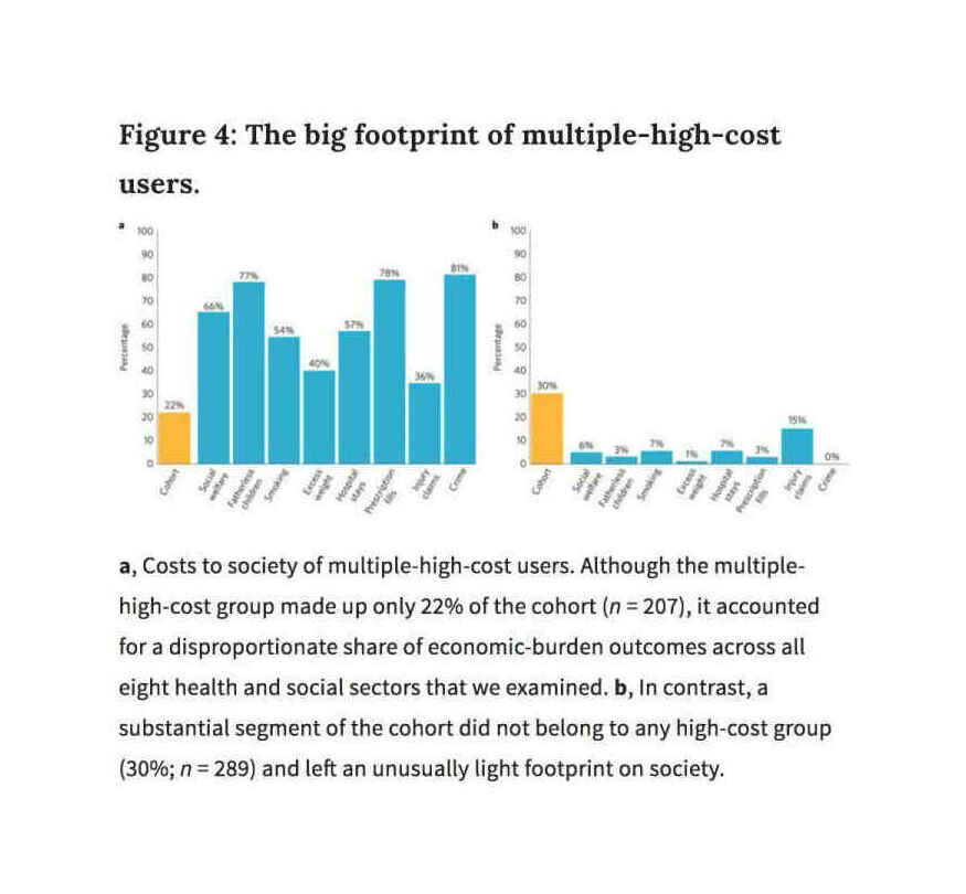

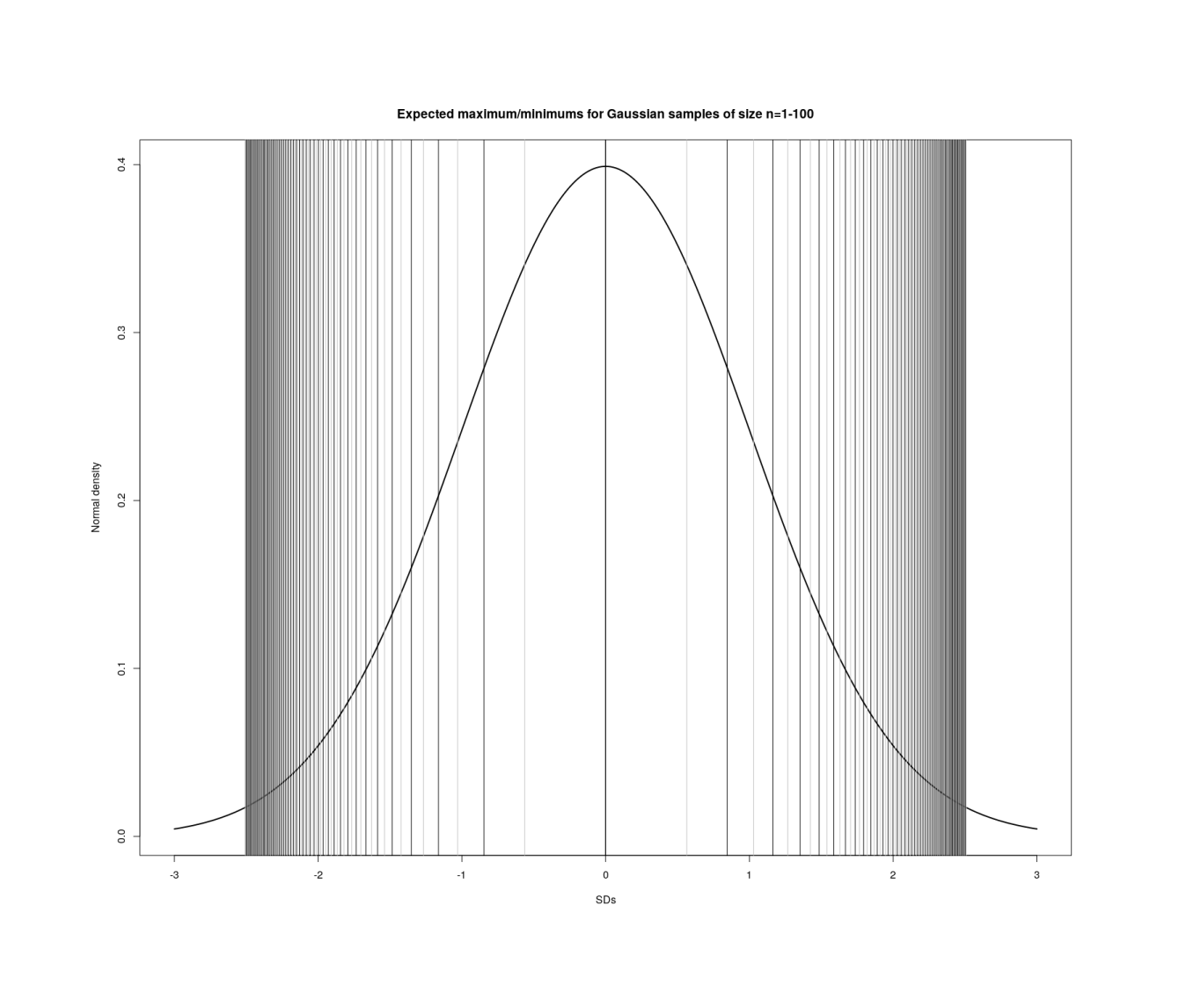
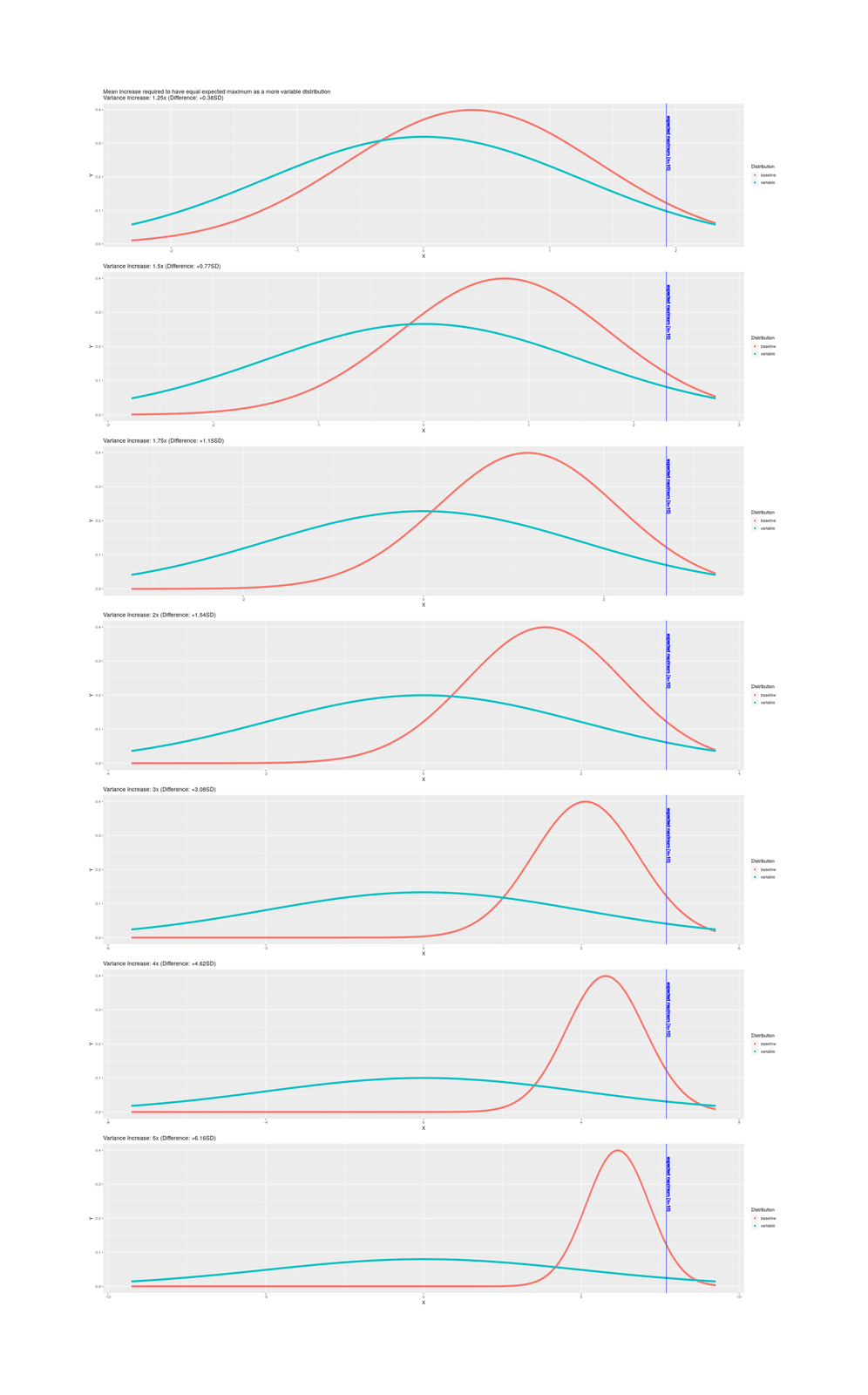
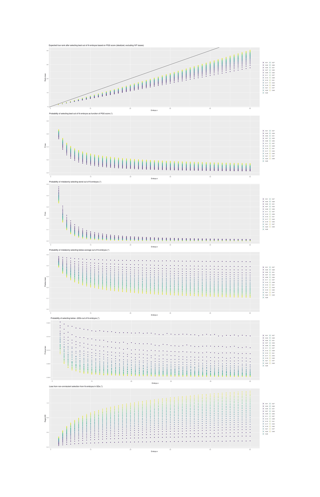


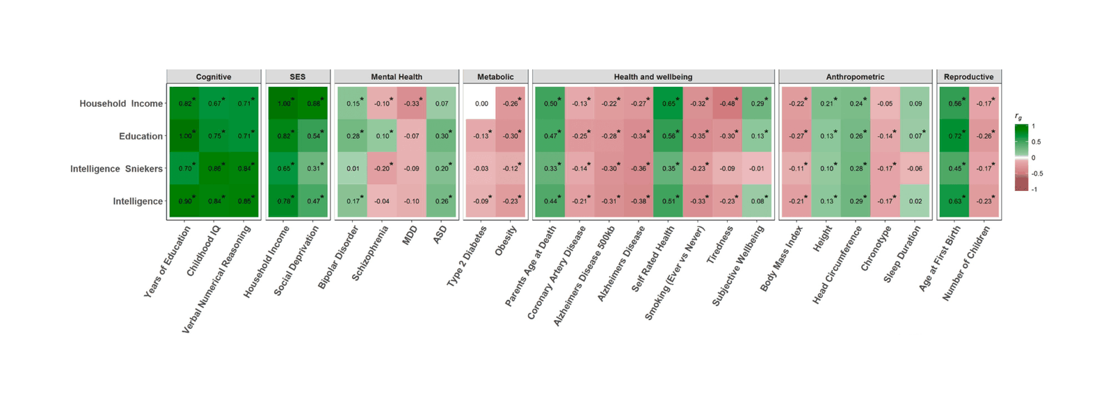
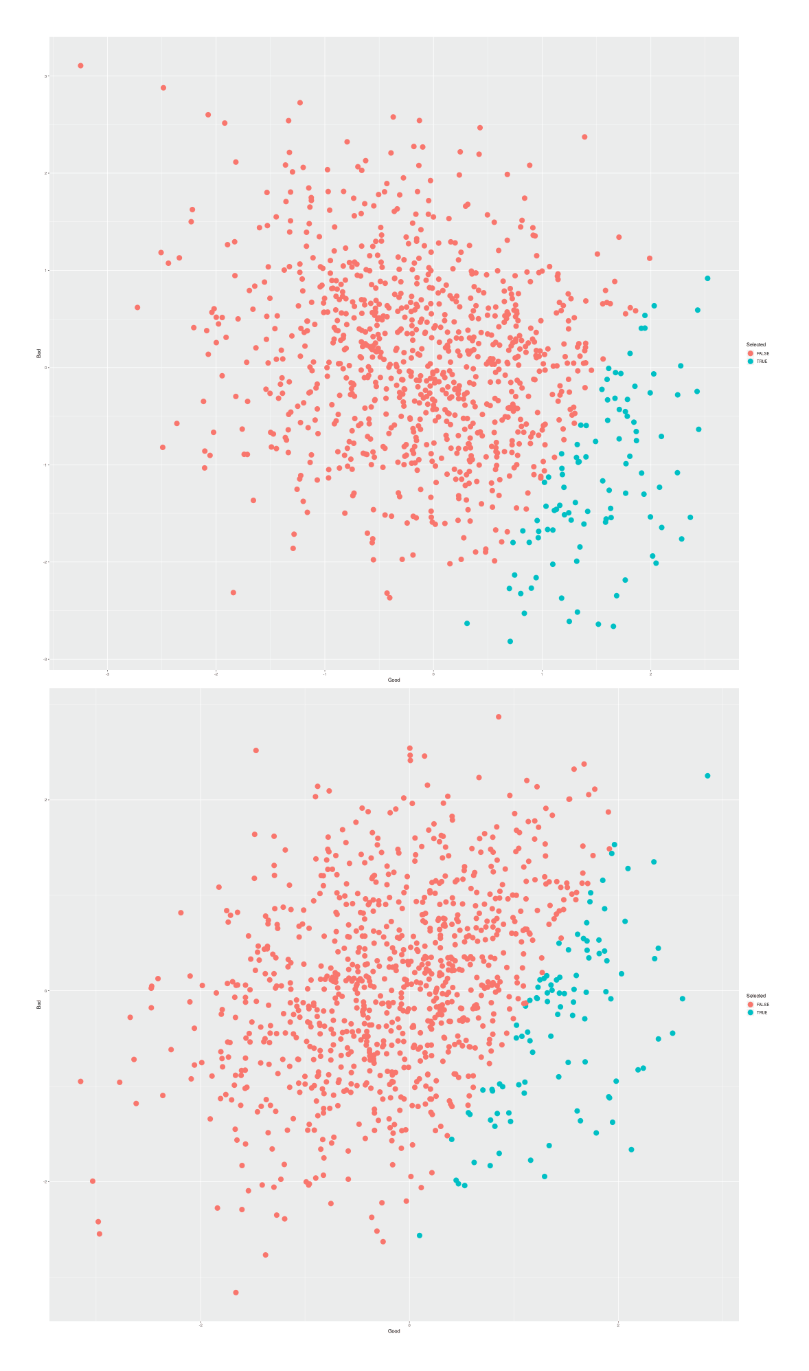


. Each box is divided into 100 squares, each representing the genotype of a locus. The squares are colored white if the person carries two non-risk alleles at a locus, blue if they carry one risk allele, and red if they carry two risk alleles. Each risk allele has frequency of 0.1 and contributes equal risk to disease. Heritability for the disease is 0.5, and disease risk is 0.01. The total number of risk alleles in the risk profile is listed at the top of each box. An average person in the population carries 20 risk alleles; thus, controls all carry risk alleles, but usually not as many as cases. Precision medicine may depend on matching genomic profiles to drug treatments. If the first row represents 10% of variants in 'core' genes, there is also considerable heterogeneity in risk profiles between people. Heterogeneity increases with the number of risk loci contributing to disease. Varying risk allele frequencies and effect sizes have little impact on the message of the visualization.")
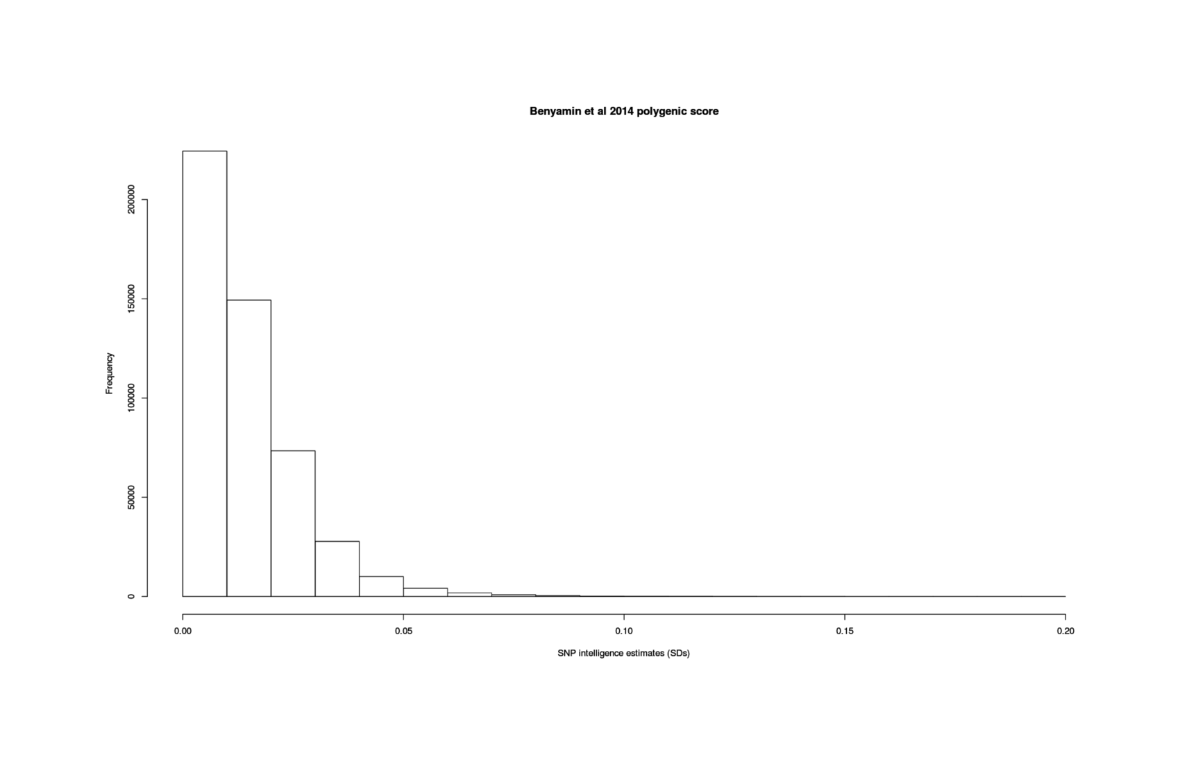
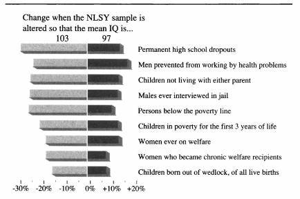
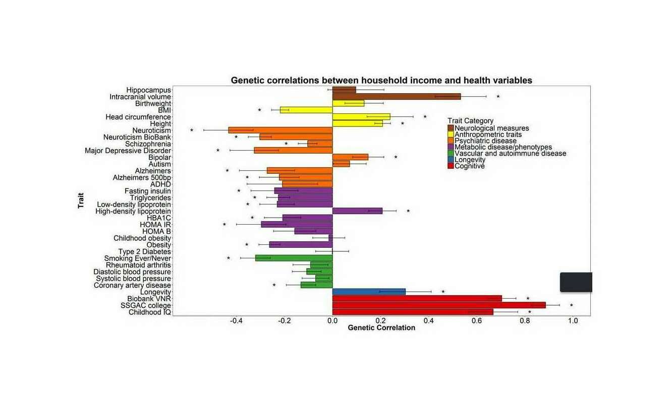
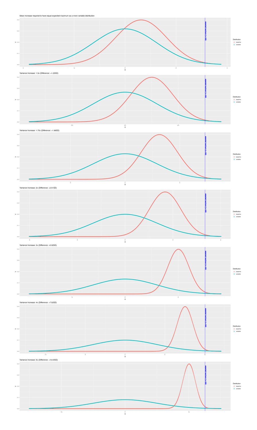
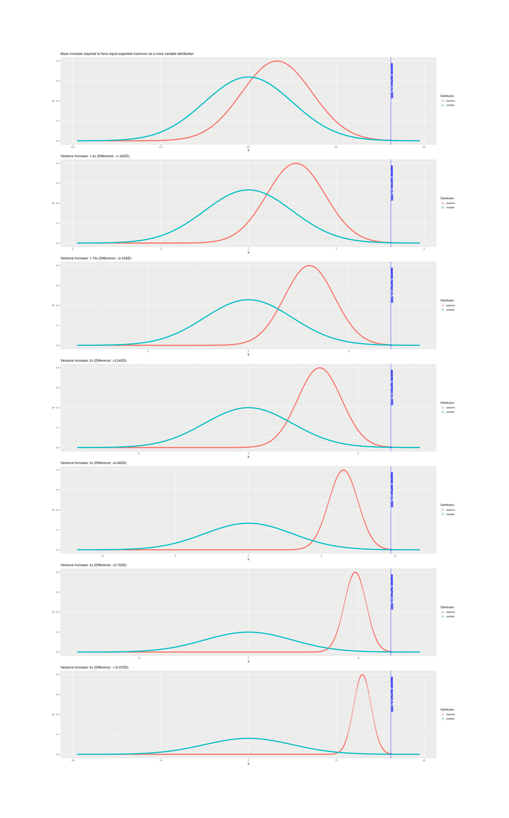
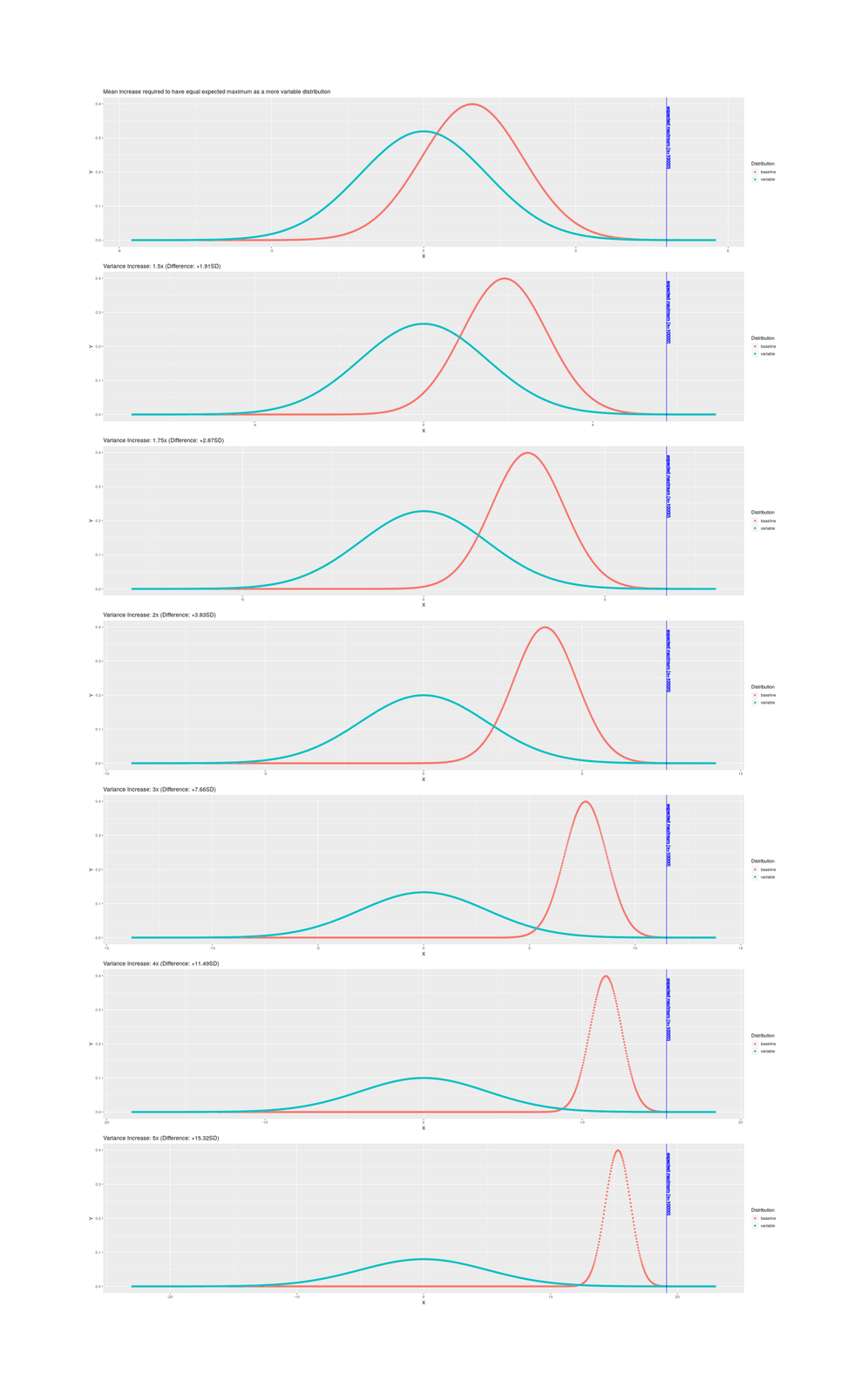
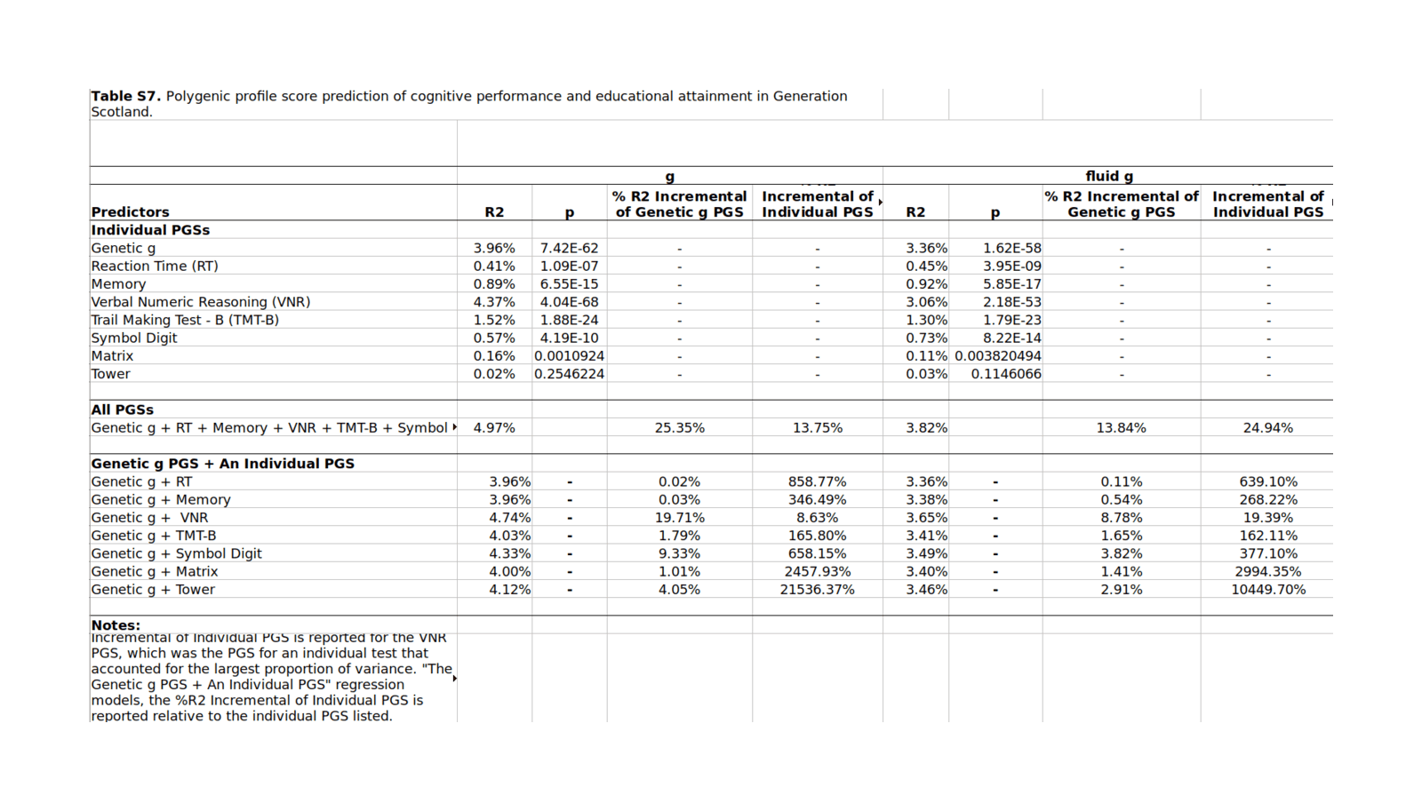
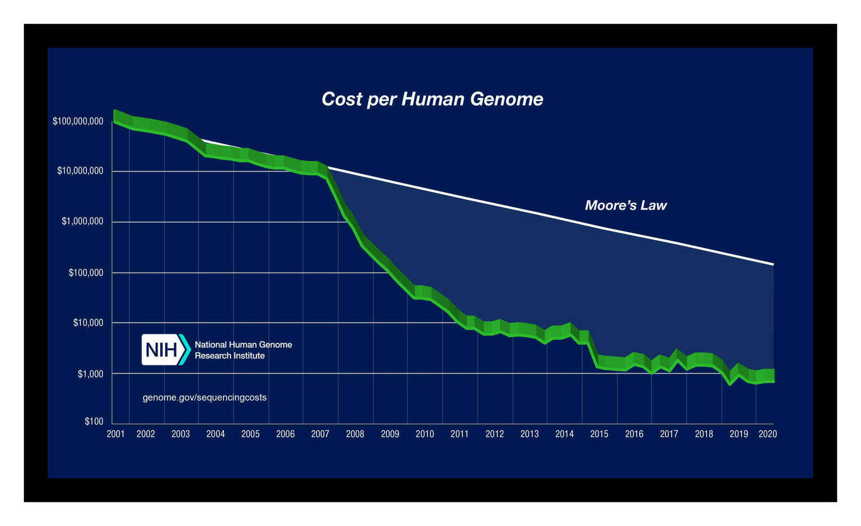
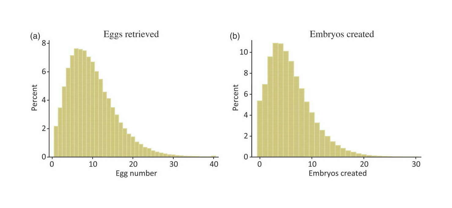
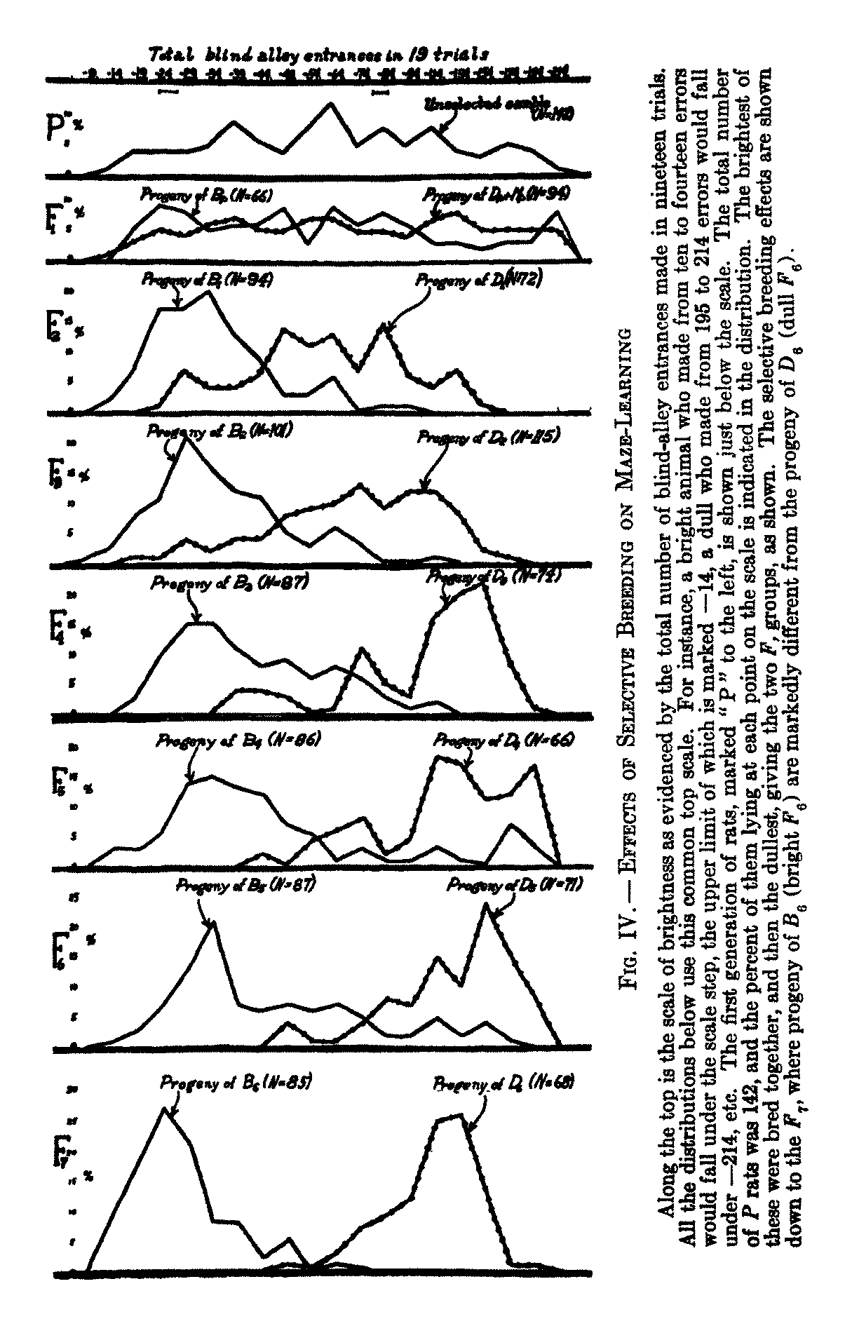
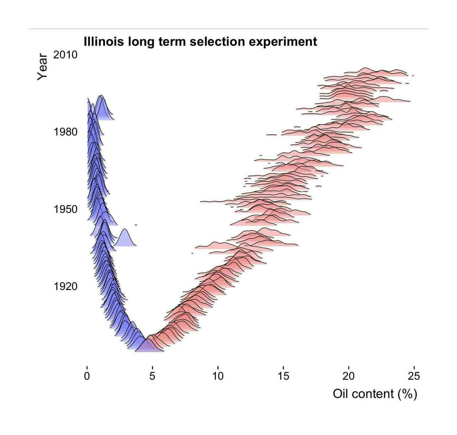