Dual n-Back Meta-Analysis
Does DNB increase IQ? What factors affect the studies? Probably not: gains are driven by studies with weakest methodology like apathetic control groups.
I meta-analyze the >19 studies up to 2016 which measure IQ after an n-back intervention, finding (over all studies) a net gain (medium-sized) on the post-training IQ tests.
The size of this increase on IQ test score correlates highly with the methodological concern of whether a study used active or passive control groups. This indicates that the medium effect size is due to methodological problems and that n-back training does not increase subjects’ underlying fluid intelligence but the gains are due to the motivational effect of passive control groups (who did not train on anything) not trying as hard as the n-back-trained experimental groups on the post-tests. The remaining studies using active control groups find a small positive effect (but this may be due to matrix-test-specific training, undetected publication bias, smaller motivational effects, etc.)
I also investigate several other n-back claims, criticisms, and indicators of bias, finding:
payment reducing performance claim: possible
dose-response relationship of n-back training time & IQ gains claim: not found
kind of n-back matters: not found
publication bias criticism: not found
speeding of IQ tests criticism: not found
Dual n-Back (DNB) is a working memory task which stresses holding several items in memory and quickly updating them. Developed for cognitive testing batteries, DNB has been repurposed for cognitive training, starting with the first study Jaeggi et al 2008, which found that training dual n-back increases scores on an IQ test for healthy young adults. If this result were true and influenced underlying intelligence (with its many correlates such as higher income or educational achievement), it would be an unprecedented result of inestimable social value and practical impact, and so is worth investigating in detail. In my DNB FAQ, I discuss a list of post-2008 experiments investigating how much and whether practicing dual n-back can increase IQ; they conflict heavily, with some finding large gains and others finding gains which are not statistically-significant or no gain at all.
What is one to make of these studies? When one has multiple quantitative studies going in both directions, one resorts to a meta-analysis: we pool the studies with their various sample sizes and effect sizes and get some overall answer - do a bunch of small positive studies outweigh a few big negative ones? Or vice versa? Or any mix thereof? Unfortunately, when I began compiling studies 2011–201313ya no one has done one for n-back & IQ already; the existing study, “Is Working Memory Training Effective? A Meta-Analytic Review” (Melby-Lervåg & Hulme 201313ya), covers working memory in general, to summarize:
However, a recent meta-analysis by Melby-Lervåg and Hulme (in press) indicates that even when considering published studies, few appropriately-powered empirical studies have found evidence for transfer from various WM training programs to fluid intelligence. Melby-Lervåg and Hulme reported that WM training showed evidence of transfer to verbal and spatial WM tasks (d = .79 and .52, respectively). When examining the effect of WM training on transfer to nonverbal abilities tests in 22 comparisons across 20 studies, they found an effect of d = .19. Critically, a moderator analysis showed that there was no effect (d = .00) in the 10 comparisons that used a treated control group, and there was a medium effect (d = .38) in the 12 comparisons that used an untreated control group.
Similar results were found by the later WM meta-analysis Schwaighofer et al 2015 and Melby-Lervåg et al 2016, and for executive function by Kassai et al 2019. (Commentary: Redick 2019.) I’m not as interested in near WM transfer from n-back training—as the Melby-Lervåg & Hulme 201313ya meta-analysis confirms, it surely does—but in the transfer with many more ramifications, transfer to IQ as measured by a matrix test. So in early 201214ya, I decided to start a meta-analysis of my own. My method & results differ from the later 201412ya DNB meta-analysis by Au & Jaeggi et al (Bayesian re-analysis) and the broad Lampit et al 2014 meta-analysis of all computer-training.
For background on conducting meta-analyses, I am using chapter 9 of part 2 of the Cochrane Collaboration’s Cochrane Handbook for Systematic Reviews of Interventions. For the actual statistical analysis, I am using the metafor package for the R language.
Literature Search
The hard part of a meta-analysis is doing a thorough literature search, but the FAQ sections represent a de facto literature search. I started the DNB FAQ in March 200917ya after reading through all available previous discussions, and have kept it up to date with the results of discussions on the DNB ML, along with alerts from Google Alerts, Google Scholar, and PubMed alerts. The corresponding authors of most of the candidate studies and Chandra Basak have been contacted with the initial list of candidate studies and asked for additional suggestions; none had a useful suggestion.
In addition, in June 201313ya I searched for "n-back" AND ("fluid intelligence" OR "IQ") in Google Scholar & PubMed. PubMed yielded no new studies; Scholar yielded Jaeggi’s 200521ya thesis. Finally, I searched ProQuest Dissertations & Theses Full Text (master’s theses & doctoral dissertations) for “n-back” and “n-back intelligence”, which turned up no new works.
Data
The candidate studies:
-
Excluded for using non-adaptive n-back and not administering an IQ post-test.
Preece 2011
Zhong 2011
Jaeggi 201214ya?
Takeuchi et al 2012
Rudebeck 2012
Thompson et al 2013
Heinzel et al 2013
Smith et al 2013
Nussbaumer et al 2013
Oelhafen et al 2013
Clouter 2013
Sprenger et al 2013
Jaeggi et al 2013
Colom et al 2013
Savage 2013
Stepankova et al 2013
Minear et al 2013
Katz et al 2013
Burki et al 2014
Pugin et al 2014
Schmiedek et al 2014
Horvat 2014
Heffernan 2014
Hancock 2013
Loosli et al 2015 (supplement):
excluded because both groups received n-back training, the experimental difference being additional interference, with near-identical improvements to all measured tasks.
Waris et al 2015
Baniqued et al 2015
Kuper & Karbach 2015
Zając-Lamparska & Trempała 2016
excluded: n-back experimental group was non-adaptive (single 1/2-back)
Lindeløv et al 2016
Schwarb et al 2015
Studer-Luethi et al 2015
excluded because did not report means/SDs for RPM scores
Minear et al 2016
Tayeri et al 2016: excluded for being quasi-experimental
Studer-Luethi et al 2016: found no transfer to the Ravens; but did not report the summary statistics so can’t be included
Variables:
activemoderator variable: whether a control group was no-contact or trained on some other task.IQ type:
BOMAT
Raven’s Advanced Progressive Matrices (RAPM)
Raven’s Standard Progressive Matrices (SPM)
other (eg. WAIS or WASI, Cattell’s Culture Fair Intelligence Test/CFIT, TONI)
record speed of IQ test: minutes allotted (upper bound if more details are given; if no time limits, default to 30 minutes since no subjects take longer)
n-back type:
dual n-back (audio & visual modalities simultaneously)
single n-back (visual modality)
single n-back (audio modality)
mixed n-back (eg. audio or visual in each block, alternating or at random)
paid: expected value of total payment in dollars, converted if necessary; if a paper does not mention payment or compensation, I assume 0 (likewise subjects receiving course credit or extra credit - so common in psychology studies that there must not be any effect), and if the rewards are of real but small value (eg. “For each correct response, participants earned points that they could cash in for token prizes such as pencils or stickers.”), I code as 1.
country: what country the subjects are from/trained in (suggested by Au et al 201412ya)
Table
The data from the surviving studies:
year |
study |
Publication |
n.e |
mean.e |
sd.e |
n.c |
mean.c |
sd.c |
active |
training |
IQ |
speed |
N.back |
paid |
country |
|---|---|---|---|---|---|---|---|---|---|---|---|---|---|---|---|
2008 |
Jaeggi1.8 |
Jaeggi1 |
4 |
14 |
2.928 |
8 |
12.13 |
2.588 |
FALSE |
200 |
0 |
10 |
0 |
0 |
Switzerland |
2008 |
Jaeggi1.8 |
Jaeggi1 |
4 |
14 |
2.928 |
7 |
12.86 |
1.46 |
TRUE |
200 |
0 |
10 |
0 |
0 |
Switzerland |
2008 |
Jaeggi1.12 |
Jaeggi1 |
11 |
9.55 |
1.968 |
11 |
8.73 |
3.409 |
FALSE |
300 |
1 |
10 |
0 |
0 |
Switzerland |
2008 |
Jaeggi1.17 |
Jaeggi1 |
8 |
10.25 |
2.188 |
8 |
8 |
1.604 |
FALSE |
425 |
1 |
10 |
0 |
0 |
Switzerland |
2008 |
Jaeggi1.19 |
Jaeggi1 |
7 |
14.71 |
3.546 |
8 |
13.88 |
3.643 |
FALSE |
475 |
1 |
20 |
0 |
0 |
Switzerland |
2009 |
Qiu |
Qiu |
9 |
132.1 |
3.2 |
10 |
130 |
5.3 |
FALSE |
250 |
2 |
25 |
0 |
0 |
China |
2009 |
polar |
Marcek1 |
13 |
32.76 |
1.83 |
8 |
25.12 |
9.37 |
FALSE |
360 |
0 |
30 |
0 |
0 |
Czech |
2010 |
Jaeggi2.1 |
Jaeggi2 |
21 |
13.67 |
3.17 |
21.5 |
11.44 |
2.58 |
FALSE |
370 |
0 |
16 |
1 |
91 |
USA |
2010 |
Jaeggi2.2 |
Jaeggi2 |
25 |
12.28 |
3.09 |
21.5 |
11.44 |
2.58 |
FALSE |
370 |
0 |
16 |
0 |
20 |
USA |
2010 |
Stephenson.1 |
Stephenson |
14 |
17.54 |
0.76 |
9.3 |
15.50 |
0.99 |
TRUE |
400 |
1 |
10 |
0 |
0.44 |
USA |
2010 |
Stephenson.2 |
Stephenson |
14 |
17.54 |
0.76 |
8.6 |
14.08 |
0.65 |
FALSE |
400 |
1 |
10 |
0 |
0.44 |
USA |
2010 |
Stephenson.3 |
Stephenson |
14.5 |
15.34 |
0.90 |
9.3 |
15.50 |
0.99 |
TRUE |
400 |
1 |
10 |
1 |
0.44 |
USA |
2010 |
Stephenson.4 |
Stephenson |
14.5 |
15.34 |
0.90 |
8.6 |
14.08 |
0.65 |
FALSE |
400 |
1 |
10 |
1 |
0.44 |
USA |
2010 |
Stephenson.5 |
Stephenson |
12.5 |
15.32 |
0.83 |
9.3 |
15.50 |
0.99 |
TRUE |
400 |
1 |
10 |
2 |
0.44 |
USA |
2010 |
Stephenson.6 |
Stephenson |
12.5 |
15.32 |
0.83 |
8.6 |
14.08 |
0.65 |
FALSE |
400 |
1 |
10 |
2 |
0.44 |
USA |
2011 |
Chooi.1.1 |
Chooi |
4.5 |
12.7 |
2 |
15 |
13.3 |
1.91 |
TRUE |
240 |
1 |
20 |
0 |
0 |
USA |
2011 |
Chooi.1.2 |
Chooi |
4.5 |
12.7 |
2 |
22 |
11.3 |
2.59 |
FALSE |
240 |
1 |
20 |
0 |
0 |
USA |
2011 |
Chooi.2.1 |
Chooi |
6.5 |
12.1 |
2.81 |
11 |
13.4 |
2.7 |
TRUE |
600 |
1 |
20 |
0 |
0 |
USA |
2011 |
Chooi.2.2 |
Chooi |
6.5 |
12.1 |
2.81 |
23 |
11.9 |
2.64 |
FALSE |
600 |
1 |
20 |
0 |
0 |
USA |
2011 |
Jaeggi3 |
Jaeggi3 |
32 |
16.94 |
4.75 |
30 |
16.2 |
5.1 |
TRUE |
287 |
2 |
10 |
1 |
1 |
USA |
2011 |
Kundu1 |
Kundu1 |
3 |
31 |
1.73 |
3 |
30.3 |
4.51 |
TRUE |
1000 |
1 |
40 |
0 |
0 |
USA |
2011 |
Schweizer |
Schweizer |
29 |
27.07 |
2.16 |
16 |
26.5 |
4.5 |
TRUE |
463 |
2 |
30 |
0 |
0 |
UK |
2011 |
Zhong.1.05d |
Zhong |
17.6 |
21.38 |
1.71 |
8.8 |
21.85 |
2.6 |
FALSE |
125 |
1 |
30 |
0 |
0 |
China |
2011 |
Zhong.1.05s |
Zhong |
17.6 |
22.83 |
2.5 |
8.8 |
21.85 |
2.6 |
FALSE |
125 |
1 |
30 |
0 |
0 |
China |
2011 |
Zhong.1.10d |
Zhong |
17.6 |
22.21 |
2.3 |
8.8 |
21 |
1.94 |
FALSE |
250 |
1 |
30 |
0 |
0 |
China |
2011 |
Zhong.1.10s |
Zhong |
17.6 |
23.12 |
1.83 |
8.8 |
21 |
1.94 |
FALSE |
250 |
1 |
30 |
0 |
0 |
China |
2011 |
Zhong.1.15d |
Zhong |
17.6 |
24.12 |
1.83 |
8.8 |
23.78 |
1.48 |
FALSE |
375 |
1 |
30 |
0 |
0 |
China |
2011 |
Zhong.1.15s |
Zhong |
17.6 |
25.11 |
1.45 |
8.8 |
23.78 |
1.48 |
FALSE |
375 |
1 |
30 |
0 |
0 |
China |
2011 |
Zhong.1.20d |
Zhong |
17.6 |
23.06 |
1.48 |
8.8 |
23.38 |
1.56 |
FALSE |
500 |
1 |
30 |
0 |
0 |
China |
2011 |
Zhong.1.20s |
Zhong |
17.6 |
23.06 |
3.15 |
8.8 |
23.38 |
1.56 |
FALSE |
500 |
1 |
30 |
0 |
0 |
China |
2011 |
Zhong.2.15s |
Zhong |
18.5 |
6.89 |
0.99 |
18.5 |
5.15 |
2.01 |
FALSE |
375 |
1 |
30 |
0 |
0 |
China |
2011 |
Zhong.2.19s |
Zhong |
18.5 |
6.72 |
1.07 |
18.5 |
5.35 |
1.62 |
FALSE |
475 |
1 |
30 |
0 |
0 |
China |
2012 |
Jaušovec |
Jaušovec |
14 |
32.43 |
5.65 |
15 |
29.2 |
6.34 |
TRUE |
1800 |
1 |
8.3 |
0 |
0 |
Slovenia |
2012 |
Kundu2 |
Kundu2 |
11 |
10.81 |
2.32 |
12 |
9.5 |
2.02 |
TRUE |
1000 |
1 |
10 |
0 |
0 |
USA |
2012 |
Redick.1 |
Redick |
12 |
6.25 |
3.08 |
20 |
6 |
3 |
FALSE |
700 |
1 |
10 |
0 |
204.3 |
USA |
2012 |
Redick.2 |
Redick |
12 |
6.25 |
3.08 |
29 |
6.24 |
3.34 |
TRUE |
700 |
1 |
10 |
0 |
204.3 |
USA |
2012 |
Rudebeck |
Rudebeck |
27 |
9.52 |
2.03 |
28 |
7.75 |
2.53 |
FALSE |
400 |
0 |
10 |
0 |
0 |
UK |
2012 |
Salminen |
Salminen |
13 |
13.7 |
2.2 |
9 |
10.9 |
4.3 |
FALSE |
319 |
1 |
20 |
0 |
55 |
Germany |
2012 |
Takeuchi |
Takeuchi |
41 |
31.9 |
0.4 |
20 |
31.2 |
0.9 |
FALSE |
270 |
1 |
30 |
0 |
0 |
Japan |
2013 |
Clouter |
Clouter |
18 |
30.84 |
4.11 |
18 |
28.83 |
2.68 |
TRUE |
400 |
3 |
12.5 |
0 |
115 |
Canada |
2013 |
Colom |
Colom |
28 |
37.25 |
6.23 |
28 |
35.46 |
8.26 |
FALSE |
720 |
1 |
20 |
0 |
204 |
Spain |
2013 |
Heinzel.1 |
Heinzel |
15 |
24.53 |
2.9 |
15 |
23.07 |
2.34 |
FALSE |
540 |
2 |
7.5 |
1 |
129 |
Germany |
2013 |
Heinzel.2 |
Heinzel |
15 |
17 |
3.89 |
15 |
15.87 |
3.13 |
FALSE |
540 |
2 |
7.5 |
1 |
129 |
Germany |
2013 |
Jaeggi.4 |
Jaeggi4 |
25 |
14.96 |
2.7 |
13.5 |
14.74 |
2.8 |
TRUE |
500 |
1 |
30 |
0 |
0 |
USA |
2013 |
Jaeggi.4 |
Jaeggi4 |
26 |
15.23 |
2.44 |
13.5 |
14.74 |
2.8 |
TRUE |
500 |
1 |
30 |
2 |
0 |
USA |
2013 |
Oelhafen |
Oelhafen |
28 |
18.7 |
3.75 |
15 |
19.9 |
4.7 |
FALSE |
350 |
0 |
45 |
0 |
54 |
Switzerland |
2013 |
Smith.1 |
Smith |
5 |
11.5 |
2.99 |
9 |
11.9 |
1.58 |
FALSE |
340 |
1 |
10 |
0 |
3.9 |
UK |
2013 |
Smith.2 |
Smith |
5 |
11.5 |
2.99 |
20 |
12.15 |
2.749 |
TRUE |
340 |
1 |
10 |
0 |
3.9 |
UK |
2013 |
Sprenger.1 |
Sprenger |
34 |
9.76 |
3.68 |
18.5 |
9.95 |
3.42 |
TRUE |
410 |
1 |
10 |
1 |
100 |
USA |
2013 |
Sprenger.2 |
Sprenger |
34 |
9.24 |
3.34 |
18.5 |
9.95 |
3.42 |
TRUE |
205 |
1 |
10 |
1 |
100 |
USA |
2013 |
Thompson.1 |
Thompson |
10 |
13.2 |
0.67 |
19 |
12.7 |
0.62 |
FALSE |
800 |
1 |
25 |
0 |
740 |
USA |
2013 |
Thompson.2 |
Thompson |
10 |
13.2 |
0.67 |
19 |
13.3 |
0.5 |
TRUE |
800 |
1 |
25 |
0 |
740 |
USA |
2013 |
Vartanian |
Vartanian |
17 |
11.18 |
2.53 |
17 |
10.41 |
2.24 |
TRUE |
60 |
1 |
10 |
1 |
0 |
Canada |
2013 |
Savage |
Savage |
23 |
11.61 |
2.5 |
27 |
11.21 |
2.5 |
TRUE |
625 |
1 |
20 |
0 |
0 |
Canada |
2013 |
Stepankova.1 |
Stepankova |
20 |
20.25 |
3.77 |
12.5 |
17.04 |
5.02 |
FALSE |
250 |
3 |
30 |
1 |
29 |
Czech |
2013 |
Stepankova.2 |
Stepankova |
20 |
21.1 |
2.95 |
12.5 |
17.04 |
5.02 |
FALSE |
500 |
3 |
30 |
1 |
29 |
Czech |
2013 |
Nussbaumer |
Nussbaumer |
29 |
13.69 |
2.54 |
27 |
11.89 |
2.24 |
TRUE |
450 |
1 |
30 |
0 |
0 |
Switzerland |
2014 |
Burki.1 |
Burki |
11 |
37.41 |
6.43 |
20 |
35.95 |
7.55 |
TRUE |
300 |
1 |
30 |
1 |
0 |
Switzerland |
2014 |
Burki.2 |
Burki |
11 |
37.41 |
6.43 |
21 |
36.86 |
6.55 |
FALSE |
300 |
1 |
30 |
1 |
0 |
Switzerland |
2014 |
Burki.3 |
Burki |
11 |
28.86 |
7.10 |
20 |
31.20 |
6.67 |
TRUE |
300 |
2 |
30 |
1 |
0 |
Switzerland |
2014 |
Burki.4 |
Burki |
11 |
28.86 |
7.10 |
23 |
27.61 |
6.82 |
FALSE |
300 |
2 |
30 |
1 |
0 |
Switzerland |
2014 |
Pugin |
Pugin |
14 |
40.29 |
2.30 |
15 |
41.33 |
1.97 |
FALSE |
600 |
3 |
30 |
1 |
1 |
Switzerland |
2014 |
Horvat |
Horvat |
14 |
48 |
5.68 |
15 |
47 |
7.49 |
FALSE |
225 |
2 |
45 |
0 |
0 |
Slovenia |
2014 |
Heffernan |
Heffernan |
9 |
32.78 |
2.91 |
10 |
31 |
3.06 |
TRUE |
450 |
3 |
20 |
0 |
140 |
Canada |
2013 |
Hancock |
Hancock |
20 |
9.32 |
3.47 |
20 |
10.44 |
4.35 |
TRUE |
810 |
1 |
30 |
1 |
50 |
USA |
2015 |
Waris |
Waris |
15 |
16.4 |
2.8 |
16 |
15.9 |
3.0 |
TRUE |
675 |
3 |
30 |
0 |
76 |
Finland |
2015 |
Baniqued |
Baniqued |
42 |
10.125 |
3.0275 |
45 |
10.25 |
3.2824 |
TRUE |
240 |
1 |
10 |
0 |
700 |
USA |
2015 |
Kuper.1 |
Kuper |
18 |
23.6 |
6.1 |
9 |
20.7 |
7.3 |
FALSE |
150 |
1 |
20 |
1 |
45 |
Germany |
2015 |
Kuper.2 |
Kuper |
18 |
24.9 |
5.5 |
9 |
20.7 |
7.3 |
FALSE |
150 |
1 |
20 |
0 |
45 |
Germany |
2016 |
Lindeløv.1 |
Lindeløv |
9 |
10.67 |
2.5 |
9 |
9.89 |
3.79 |
TRUE |
260 |
1 |
10 |
3 |
0 |
Denmark |
2016 |
Lindeløv.2 |
Lindeløv |
8 |
3.25 |
2.71 |
9 |
4.11 |
1.36 |
TRUE |
260 |
1 |
10 |
3 |
0 |
Denmark |
2015 |
Schwarb.1 |
Schwarb |
26 |
0.11 |
2.5 |
26 |
0.69 |
3.2 |
FALSE |
480 |
1 |
10 |
3 |
80 |
USA |
2015 |
Schwarb.2.1 |
Schwarb |
22 |
0.23 |
2.5 |
10.5 |
-0.36 |
2.1 |
FALSE |
480 |
1 |
10 |
1 |
80 |
USA |
2015 |
Schwarb.2.2 |
Schwarb |
23 |
0.91 |
3.1 |
10.5 |
-0.36 |
2.1 |
FALSE |
480 |
1 |
10 |
2 |
80 |
USA |
2016 |
Heinzel.1 |
Heinzel.2 |
15 |
17.73 |
1.20 |
14 |
16.43 |
1.00 |
FALSE |
540 |
2 |
7.5 |
1 |
1 |
Germany |
2016 |
Lawlor-Savage |
Lawlor |
27 |
11.48 |
2.98 |
30 |
11.02 |
2.34 |
TRUE |
391 |
1 |
20 |
0 |
0 |
Canada |
2016 |
Minear.1 |
Minear |
15.5 |
24.1 |
4.5 |
26 |
24 |
5.1 |
TRUE |
400 |
1 |
15 |
1 |
300 |
USA |
2016 |
Minear.2 |
Minear |
15.5 |
24.1 |
4.5 |
37 |
22.8 |
4.6 |
TRUE |
400 |
1 |
15 |
1 |
300 |
USA |
Analysis
The result of the meta-analysis:
Random-Effects Model (k = 74; tau^2 estimator: REML)

tau^2 (estimated amount of total heterogeneity): 0.1103 (SE = 0.0424)
tau (square root of estimated tau^2 value):      0.3321
I^2 (total heterogeneity / total variability):   43.83%
H^2 (total variability / sampling variability):  1.78

Test for Heterogeneity:
Q(df = 73) = 144.2388, p-val < .0001

Model Results:

estimate       se     zval     pval    ci.lb    ci.ub
  0.3460   0.0598   5.7836   <.0001   0.2288   0.4633
To depict the random-effects model in a more graphic form, we use the “forest plot”:
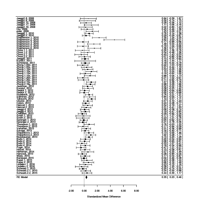
forest(res1, slab = paste(dnb$study, dnb$year, sep = ", "))
The overall effect is somewhat strong. But there seems to be substantial differences between studies: this heterogeneity may be what is showing up as a high τ2 and i2; and indeed, if we look at the computed SMDs, we see one sample with d = 2.59 (!) and some instances of d < 0. The high heterogeneity means that the fixed-effects model is inappropriate, as clearly the studies are not all measuring the same effect, so we use a random-effects.
The confidence interval excludes zero, so one might conclude that n-back does increase IQ scores. From a Bayesian standpoint, it’s worth pointing out that this is not nearly as conclusive as it seems, for several reasons:
Published research can be weak (see the Replication Crisis); meta-analyses are generally believed to be biased towards larger effects due to systematic biases like publication bias
our prior that any particular intervention would increase the underlying genuine fluid intelligence is extremely small, as scores or hundreds of attempts to increase IQ over the past century have all eventually turned out to be failures, with few exceptions (eg. pre-natal iodine or iron supplementation), so strong evidence is necessary to conclude that a particular attempt is one of those extremely rare exceptions. As the saying goes, “extraordinary claims require extraordinary evidence”. David Hambrick explains it informally:
…Yet I and many other intelligence researchers are skeptical of this research. Before anyone spends any more time and money looking for a quick and easy way to boost intelligence, it’s important to explain why we’re not sold on the idea…Does this [Jaeggi et al 200818ya] sound like an extraordinary claim? It should. There have been many attempts to demonstrate large, lasting gains in intelligence through educational interventions, with few successes. When gains in intelligence have been achieved, they have been modest and the result of many years of effort. For instance, in a University of North Carolina study known as the Abecedarian Early Intervention Project, children received an intensive educational intervention from infancy to age 5 designed to increase intelligence1. In follow-up tests, these children showed an advantage of six I.Q. points over a control group (and as adults, they were four times more likely to graduate from college). By contrast, the increase implied by the findings of the Jaeggi study was six I.Q. points after only six hours of training - an I.Q. point an hour. Though the Jaeggi results are intriguing, many researchers have failed to demonstrate statistically-significant gains in intelligence using other, similar cognitive training programs, like Cogmed’s… We shouldn’t be surprised if extraordinary claims of quick gains in intelligence turn out to be wrong. Most extraordinary claims are.
it’s not clear that just because IQ tests like Raven’s are valid and useful for measuring levels of intelligence, that an increase on the tests can be interpreted as an increase of intelligence; intelligence poses unique problems of its own in any attempt to show increases in the latent variable of gf rather than just the raw scores of tests (which can be, essentially, ‘gamed’). Haier 2014 analogizes claims of breakthrough IQ increases to the initial reports of cold fusion and comments:
The basic misunderstanding is assuming that intelligence test scores are units of measurement like inches or liters or grams. They are not. Inches, liters and grams are ratio scales where zero means zero and 100 units are twice 50 units. Intelligence test scores estimate a construct using interval scales and have meaning only relative to other people of the same age and sex. People with high scores generally do better on a broad range of mental ability tests, but someone with an IQ score of 130 is not 30% smarter then someone with an IQ score of 100…This makes simple interpretation of intelligence test score changes impossible. Most recent studies that have claimed increases in intelligence after a cognitive training intervention rely on comparing an intelligence test score before the intervention to a second score after the intervention. If there is an average change score increase for the training group that is statistically-significant (using a dependent t-test or similar statistical test), this is treated as evidence that intelligence has increased. This reasoning is correct if one is measuring ratio scales like inches, liters or grams before and after some intervention (assuming suitable and reliable instruments like rulers to avoid erroneous Cold Fusion-like conclusions that apparently were based on faulty heat measurement); it is not correct for intelligence test scores on interval scales that only estimate a relative rank order rather than measure the construct of intelligence….Studies that use a single test to estimate intelligence before and after an intervention are using less reliable and more variable scores (bigger standard errors) than studies that combine scores from a battery of tests….Speaking about science, Carl Sagan observed that extraordinary claims require extraordinary evidence. So far, we do not have it for claims about increasing intelligence after cognitive training or, for that matter, any other manipulation or treatment, including early childhood education. Small statistically-significant changes in test scores may be important observations about attention or memory or some other elemental cognitive variable or a specific mental ability assessed with a ratio scale like milliseconds, but they are not sufficient proof that general intelligence has changed.
For statistical background on how one should be measuring changes on a latent variable like intelligence and running intervention studies, see Cronbach & Furby 1970 & Moreau et al 2016; for examples of past IQ interventions which fadeout, see Protzko 2015; for examples of past IQ interventions which prove not to be on g when analyzed in a latent variable approach, see Jensen’s informal comments on the Milwaukee Project (Jensen 1989), te Nijenhuis et al 2007, te Nijenhuis et al 2014, te Nijenhuis et al 2015, Nutley et al 2011, Shipstead et al 2012, Colom et al 2013, Hayes et al 2014, Ritchie et al 2015, Estrada et al 2015, Bailey et al 2017 (and in a null, the composite score in Baniqued et al 2015).
This skeptical attitude is relevant to our examination of moderators.
Moderators
Control Groups
A major criticism of n-back studies is that the effect is being manufactured by the methodological problem of some studies using a no-contact or passive control group rather than an active control group. (Passive controls know they received no intervention and that the researchers don’t expect them to do better on the post-test, which may reduce their efforts & lower their scores.)
The review Morrison & Chein 20112 noted that no-contact control groups limited the validity of such studies, a criticism that was echoed with greater force by Shipstead, Redick, & Engle 201214ya. The Melby-Lervåg & Hulme 2013 WM training meta-analysis then confirmed that use of no-contact controls inflated the effect size estimates3, similar to Zehdner et al 2009/Sala et al 2019 results in the aged and Rapport et al 2013’s blind vs unblinded ratings in WM/executive training of ADHD or Long et al 2019’s inflation of emotional regulation benefits from DNB training, and WM training in young children (Sala & Gobet 2017a find passive control groups inflate effect sizes by g = 0.12, and are further critical in Sala & Gobet 2017b4); and consistent with the “dodo bird verdict” and the increase of d = 0.2 across many kinds of psychological therapies which was found by Lipsey & Wilson 1993 (but inconsistent with the g = 0.20 vs g = 0.26 of Lampit et al 201412ya), and De Quidt et al 2018 demonstrating strong demand effects can reach as high as d = 1 (with a mean d = 0.6, quite close to the actual passive DNB effect).
So I wondered if this held true for the subset of n-back & IQ studies. (Age is an interesting moderator in Melby-Lervåg & Hulme 201313ya, but in the following DNB & IQ studies there is only 1 study involving children - all the others are adults or young adults.) Each study has been coded appropriately, and we can ask whether it matters:
Mixed-Effects Model (k = 74; tau^2 estimator: REML)

tau^2 (estimated amount of residual heterogeneity):     0.0803 (SE = 0.0373)
tau (square root of estimated tau^2 value):             0.2834
I^2 (residual heterogeneity / unaccounted variability): 36.14%
H^2 (unaccounted variability / sampling variability):   1.57

Test for Residual Heterogeneity:
QE(df = 72) = 129.2820, p-val < .0001

Test of Moderators (coefficient(s) 1,2):
QM(df = 2) = 46.5977, p-val < .0001

Model Results:

                     estimate      se    zval    pval    ci.lb   ci.ub
factor(active)FALSE    0.4895  0.0738  6.6310  <.0001   0.3448  0.6342
factor(active)TRUE     0.1397  0.0862  1.6211  0.1050  -0.0292  0.3085
The active/control variable confirms the criticism: lack of active control groups is responsible for a large chunk of the overall effect, with the confidence intervals not overlapping. The effect with passive control groups is a medium-large d = 0.5 while with active control groups, the IQ gains shrink to a small effect (whose 95% CI does not exclude d = 0).
We can see the difference by splitting a forest plot on passive vs active:
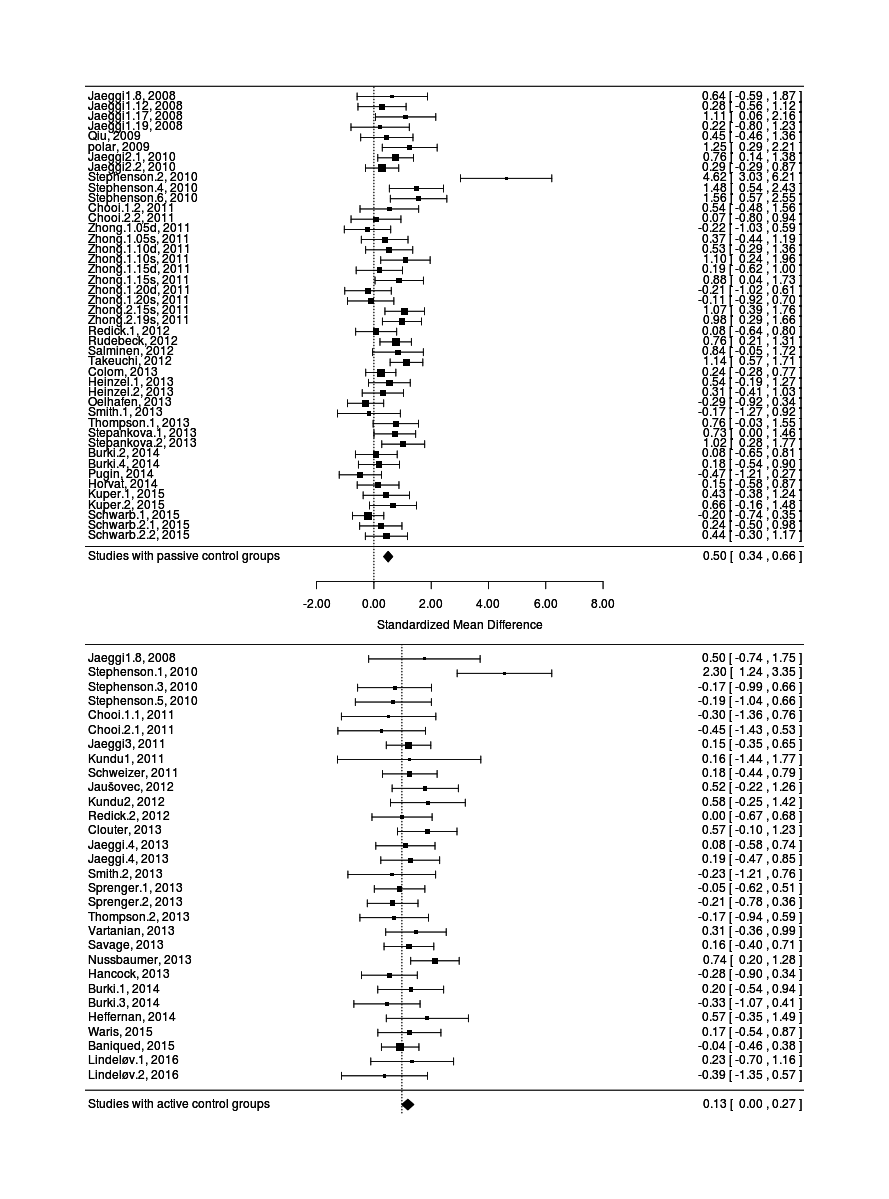
The visibly different groups of passive then active studies, plotted on the same axis
This is damaging to the case that dual n-back increases intelligence, if it’s unclear if it even increases a particular test score. Not only do the better studies find a drastically smaller effect, they are not sufficiently powered to find such a small effect at all, even aggregated in a meta-analysis, with a power of ~11%, which is dismal indeed when compared to the usual benchmark of 80%, and leads to worries that even that is too high an estimate and that the active control studies are aberrant somehow in being subject to a winner’s curse or subject to other biases. (Because many studies used convenient passive control groups and the passive effect size is 3x larger, they in aggregate are well-powered at 82%; however, we already know they are skewed upwards, so we don’t care if we can detect a biased effect or not.) In particular, Boot et al 2013 argues that active control groups do not suffice to identify the true causal effect because the subjects in the active control group can still have different expectations than the experimental group, and the group’ differing awareness & expectations can cause differing performance on tests (an example of which is demonstrated by Foroughi et al 2016); they suggest recording expectancies (somewhat similar to Redick et al 201313ya), checking for a dose-response relationship (see the following section for whether dose-response exists for dual n-back/IQ), and using different experimental designs which actively manipulate subject expectations to identify how much effects are inflated by remaining placebo/expectancy effects.
The active estimate of d = 0.14 does allow us to estimate how many subjects a simple5 two-group experiment with an active control group would require in order for it to be well-powered (80%) to detect an effect: a total n of >1600426ya subjects (805 in each group).
Training Time
Jaeggi et al 200818ya observed a dose-response to training, where those who trained the longest apparently improved the most. Ever since, this has been cited as a factor in what studies will observe gains or as an explanation why some studies did not see improvements - perhaps they just didn’t do enough training. metafor is able to look at the number of minutes subjects in each study trained for to see if there’s any clear linear relationship:
         estimate      se     zval    pval    ci.lb   ci.ub
intrcpt    0.3961  0.1226   3.2299  0.0012   0.1558  0.6365
mods      -0.0001  0.0002  -0.4640  0.6427  -0.0006  0.0004
The estimate of the relationship is that there is none at all: the estimated coefficient has a large p-value, and further, that coefficient is negative. This may seem initially implausible but if we graph the time spent training per study with the final (unweighted) effect size, we see why:
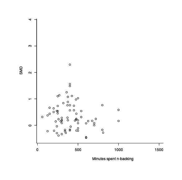
plot(dnb$training, res1$yi)
IQ Test Time
Similarly, Moody 200917ya identified the 10 minute test-time or “speeding” of the RAPM as a concern in whether far transfer actually happened; after collecting the allotted test time for the studies, we can likewise look for whether there is an inverse relationship (the more time given to subjects on the IQ test, the smaller their IQ gains):
         estimate      se     zval    pval    ci.lb   ci.ub
intrcpt    0.4197  0.1379   3.0435  0.0023   0.1494  0.6899
mods      -0.0036  0.0061  -0.5874  0.5570  -0.0154  0.0083
A tiny slope which is also non-statistically-significant; graphing the (unweighted) studies suggests as much:
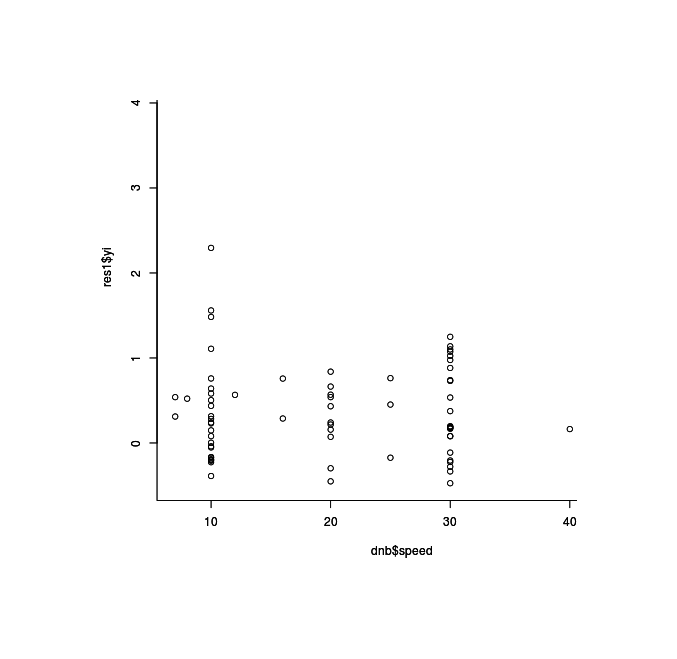
plot(dnb$speed, res1$yi)
Training Type
One question of interest both for issues of validity and for effective training is whether the existing studies show larger effects for a particular kind of n-back training: dual (visual & audio; labeled 0) or single (visual; labeled 1) or single (audio; labeled 2)? If visual single n-back turns in the largest effects, that is troubling since it’s also the one most resembling a matrix IQ test. Checking against the 3 kinds of n-back training:
Mixed-Effects Model (k = 74; tau^2 estimator: REML)

tau^2 (estimated amount of residual heterogeneity):     0.1029 (SE = 0.0421)
tau (square root of estimated tau^2 value):             0.3208
I^2 (residual heterogeneity / unaccounted variability): 41.94%
H^2 (unaccounted variability / sampling variability):   1.72

Test for Residual Heterogeneity:
QE(df = 70) = 135.5275, p-val < .0001

Test of Moderators (coefficient(s) 1,2,3,4):
QM(df = 4) = 39.1393, p-val < .0001

Model Results:

                 estimate      se     zval    pval    ci.lb   ci.ub
factor(N.back)0    0.4219  0.0747   5.6454  <.0001   0.2754  0.5684
factor(N.back)1    0.2300  0.1102   2.0876  0.0368   0.0141  0.4459
factor(N.back)2    0.4255  0.2586   1.6458  0.0998  -0.0812  0.9323
factor(N.back)3   -0.1325  0.2946  -0.4497  0.6529  -0.7099  0.4449
There are not enough studies using the other kinds of n-back to say anything conclusive other than there seem to be differences, but it’s interesting that single visual n-back has weaker results so far.
Payment/extrinsic Motivation
In a 201313ya talk, “‘Brain Training: Current Challenges and Potential Resolutions’, with Susanne Jaeggi, PhD”, Jaeggi suggests
Extrinsic reward can undermine people’s intrinsic motivation. If extrinsic reward is crucial, then its influence should be visible in our data.
I investigated payment as a moderator. Payment seems to actually be quite rare in n-back studies (in part because it’s so common in psychology to just recruit students with course credit or extra credit), and so the result is that as a moderator payment is currently a small and non-statistically-significant negative effect, whether you regress on the total payment amount or treat it as a boolean variable. More interestingly, it seems that the negative sign is being driven by payment being associated with higher-quality studies using active control groups, because when you look at the interaction, payment in a study with an active control group actually flips sign to being positive again (correlating with a bigger effect size).
More specifically, if we check payment as a binary variable, we get a decrease which is statistically-significant:
                      estimate      se     zval    pval    ci.lb   ci.ub
intrcpt                 0.4514  0.0776   5.8168  <.0001   0.2993   0.6035
as.logical(paid)TRUE   -0.2424  0.1164  -2.0828  0.0373  -0.4706  -0.0143
If we instead regress against the total payment size (logically, larger payments would discourage participants more), the effect of each additional dollar is tiny and 0 is far from excluded as the coefficient:
         estimate      se     zval    pval    ci.lb   ci.ub
intrcpt    0.3753  0.0647   5.7976  <.0001   0.2484  0.5022
paid      -0.0004  0.0004  -1.1633  0.2447  -0.0012  0.0003
Why would treating payment as a binary category yield a major result when there is only a small slope within the paid studies? It would be odd if n-back could achieve the holy grail of increasing intelligence, but the effect vanishes immediately whether you pay subjects anything, whether $1 or $1,000.
As I’ve mentioned before, the difference in effect size between active and passive control groups is quite striking, and I noticed that eg. the Redick et al 201214ya experiment paid subjects a lot of money to put up with all its tests and ensure subject retention & Thompson et al 201313ya paid a lot to put up with the fMRI machine and long training sessions, and likewise with Oelhafen et al 201313ya and Baniqued et al 201511ya etc.; so what happens if we look for an interaction?
                                 estimate      se     zval    pval    ci.lb    ci.ub
intrcpt                            0.6244  0.0971   6.4309  <.0001   0.4341   0.8147
activeTRUE                        -0.4013  0.1468  -2.7342  0.0063  -0.6890  -0.1136
as.logical(paid)TRUE              -0.2977  0.1427  -2.0860  0.0370  -0.5774  -0.0180
activeTRUE:as.logical(paid)TRUE    0.1039  0.2194   0.4737  0.6357  -0.3262   0.5340
Active control groups cuts the observed effect of n-back by more than half, as before, and payment increases the effect size, but then in studies which use active control groups and also pays subjects, the effect size increases slightly again with payment size, which seems a little curious if we buy the story about extrinsic motivation crowding out intrinsic and defeating any gains.
Biases
N-back has been presented in some popular & academic medias in an entirely uncritical & positive light: ignoring the overwhelming failure of intelligence interventions in the past, not citing the failures to replicate, and giving short schrift to the criticisms which have been made. (Examples include the NYT, WSJ, Scientific American, & Nisbett et al 2012.) One researcher told me that a reviewer savaged their work, asserting that n-back works and thus their null result meant only that they did something wrong. So it’s worth investigating, to the extent we can, whether there is a publication bias towards publishing only positive results.
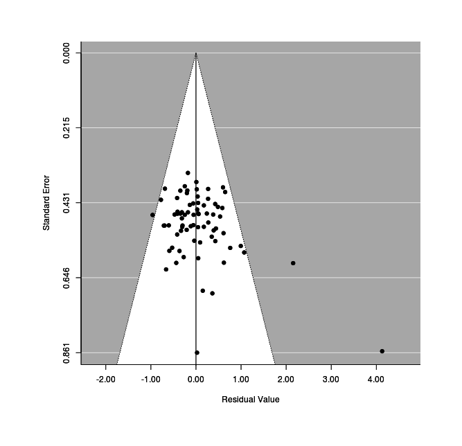
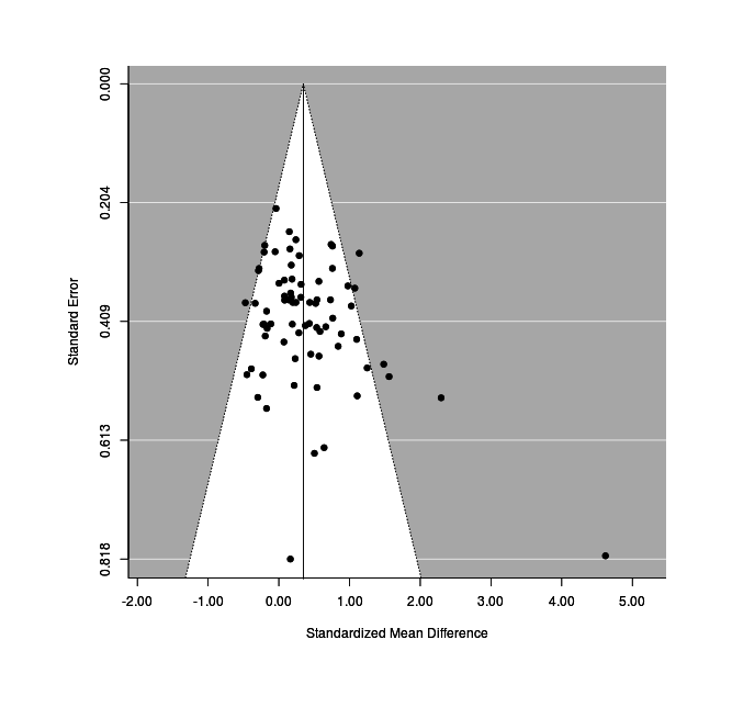
20-odd studies (some quite small) is considered medium-sized for a meta-analysis, but that many does permit us to generate funnel plots , or check for possible publication bias via the trim-and-fill method.
Funnel Plot
test for funnel plot asymmetry: z = 3.0010, p = 0.0027The asymmetry has reached statistical-significance, so let’s visualize it:

funnel(res1)
This looks reasonably good, although we see that studies are crowding the edges of the funnel. We know that the studies with active control groups show twice the effect-size of the passive control groups, is this related? If we plot the residual left after correcting for active vs passive, the funnel plot improves a lot (Stephenson remains an outlier):
Mixed-effects plot of standard error versus effect size after moderator correction.
Trim-And-Fill
The trim-and-fill estimate:
Estimated number of missing studies on the left side: 0 (SE = 4.8908)Graphing it:
funnel(tf)
Overall, the results suggest that this particular (comprehensive) collection of DNB studies does not suffer from serious publication bias after taking in account the active/passive moderator.
Notes
Going through them, I must note:
Jaeggi 200818ya: group-level data provided by Jaeggi to Redick for Redick et al 201313ya; the 8-session group included both active & passive controls, so experimental DNB group was split in half. IQ test time is based on the description in Redick et al 201214ya:
In addition, the 19-session groups were 20 min to complete BOMAT, whereas the 12- and 17-session groups received only 10 min (S. M. Jaeggi, personal communication, May 25, 201115ya). As shown in Figure 2, the use of the short time limit in the 12- and 17-session studies produced substantially lower scores than the 19-session study.
polar: control, 2nd scores: 23,27,19,15,12,35,36,34; experiment, 2nd scores: 30,35,33,33,32,30,35,33,35,33,34,30,33
Jaeggi 201016ya: used BOMAT scores; should I somehow pool RAPM with BOMAT? Control group split.
Jaeggi 201115ya: used SPM (a Raven’s); should I somehow pool the TONI?
Schweizer 201115ya: used the adjusted final scores as suggested by the authors due to potential pre-existing differences in their control & experimental groups:
…This raises the possibility that the relative gains in Gf in the training versus control groups may be to some extent an artefact of baseline differences. However, the interactive effect of transfer as a function of group remained [statistically-]significant even after more closely matching the training and control groups for pre-training RPM scores (by removing the highest scoring controls) F(1, 30) = 3.66, P = 0.032, gp2 = 0.10. The adjusted means (standard deviations) for the control and training groups were now 27.20 (1.93), 26.63 (2.60) at pre-training (t(43) = 1.29, P.0.05) and 26.50 (4.50), 27.07 (2.16) at post-training, respectively.
Stephenson data from pg79/95; means are post-scores on Raven’s. I am omitting Stephenson scores on WASI, Cattell’s Culture Fair Test, & BETA III Matrix Reasoning subset because
metafordoes not support multivariate meta-analyses and including them as separate studies would be statistically illegitimate. The active and passive control groups were split into thirds over each of the 3 n-back training regimens, and each training regimen split in half over the active & passive controls.The splitting is worth discussion. Some of these studies have multiple experimental groups, control groups, or both. A criticism of early studies was the use of no-contact control groups - the control groups did nothing except be tested twice, and it was suggested that the experimental group gains might be in part solely because they are doing a task, any task, and the control group should be doing some non-WM task as well. The WM meta-analysis Melby-Lervåg & Hulme 201313ya checked for this and found that use of no-contact control groups led to a much larger estimate of effect size than studies which did use an active control. When trying to incorporate such a multi-part experiment, one cannot just copy controls as the Cochrane Handbook points out:
One approach that must be avoided is simply to enter several comparisons into the meta-analysis when these have one or more intervention groups in common. This ‘double-counts’ the participants in the ‘shared’ intervention group(s), and creates a unit-of-analysis error due to the unaddressed correlation between the estimated intervention effects from multiple comparisons (see Chapter 9, §9.3).
Just dropping one control or experimental group weakens the meta-analysis, and may bias it as well if not done systematically. I have used one of its suggested approaches which accepts some additional error in exchange for greater power in checking this possible active versus no-contact distinction, in which we instead split the shared group:
A further possibility is to include each pair-wise comparison separately, but with shared intervention groups divided out approximately evenly among the comparisons. For example, if a trial compares 121 patients receiving acupuncture with 124 patients receiving sham acupuncture and 117 patients receiving no acupuncture, then two comparisons (of, say, 61 ‘acupuncture’ against 124 ‘sham acupuncture’, and of 60 ‘acupuncture’ against 117 ‘no intervention’) might be entered into the meta-analysis. For dichotomous outcomes, both the number of events and the total number of patients would be divided up. For continuous outcomes, only the total number of participants would be divided up and the means and standard deviations left unchanged. This method only partially overcomes the unit-of-analysis error (because the resulting comparisons remain correlated) so is not generally recommended. A potential advantage of this approach, however, would be that approximate investigations of heterogeneity across intervention arms are possible (for example, in the case of the example here, the difference between using sham acupuncture and no intervention as a control group).
Chooi: the relevant table was provided in private communication; I split each experimental group in half to pair it up with the active and passive control groups which trained the same number of days
Takeuchi et al 2012: subjects were trained on 3 WM tasks in addition to DNB for 27 days, 30-60 minutes; RAPM scores used, BOMAT & Tanaka B-type intelligence test scores omitted
Jaušovec 201214ya: IQ test time was calculated based on the description
Used were 50 test items - 25 easy (Advanced Progressive Matrices Set I - 12 items and the B Set of the Colored Progressive Matrices), and 25 difficult items (Advanced Progressive Matrices Set II, items 12-36). Participants saw a figural matrix with the lower right entry missing. They had to determine which of the four options fitted into the missing space. The tasks were presented on a computer screen (positioned about 80-100 cm in front of the respondent), at fixed 10 or 14 s interstimulus intervals. They were exposed for 6 s (easy) or 10 s (difficult) following a 2-s interval, when a cross was presented. During this time the participants were instructed to press a button on a response pad (1-4) which indicated their answer.
(25 × (6+2) + 25 × (10+2)) / 60 = 8.33 minutes.
Zhong 201115ya: “dual attention channel” task omitted, dual and single n-back scores kept unpooled and controls split across the 2; I thank Emile Kroger for his translations of key parts of the thesis. Unable to get whether IQ test was administered speeded. Zhong 201115ya appears to have replicated Jaeggi 2008’s training time.
Jonasson 201115ya omitted for lacking any measure of IQ
Preece 201115ya omitted; only the Figure Weights subtest from the WAIS was reported, but RAPM scores were taken and published in the inaccessible Palmer 2011
Kundu et al 201115ya and Kundu 201214ya have been split into 2 experiments based on the raw data provided to me by Kundu: the smaller one using the full RAPM 36-matrix 40-minute test, and the larger an 18-matrix 10-minute test. (Kundu 201214ya subsumes 201115ya, but the procedure was changed partway on Jaeggi’s advice, so they are separate results.) The final results were reported in “Strengthened effective connectivity underlies transfer of working memory training to tests of short-term memory and attention”, Kundu et al 201313ya.
Redick et al: n-back split over passive control & active control (visual search) RAPM post scores (omitted SPM and Cattell Culture-Fair Test)
Vartanian 201313ya: short n-back intervention not adaptive; I did not specify in advance that the n-back interventions had to be adaptive (possibly some of the others were not) and subjects trained for <50 minutes, so the lack of adaptiveness may not have mattered.
Heinzel et al 201313ya mentions conducting a pilot study; I contacted Heinzel and no measures like Raven’s were taken in it. The main study used both SPM and also “the Figural Relations subtest of a German intelligence test (LPS)”; as usual, I drop alternatives in favor of the more common test.
Thompson et al 201313ya; used RAPM rather than WAIS; treated the “multiple object tracking”/MOT as an active control group since it did not statistically-significantly improve RAPM scores
Smith et al 201313ya; 4 groups. Consistent with all the other studies, I have ignored the post-post-tests (a 4-week followup). To deal with the 4 groups, I have combined the Brain Age & strategy game groups into a single active control group, and then split the dual n-back group in half over the original passive control group and the new active control group.
Jaeggi 200521ya: Jaeggi et al 200818ya is not clear about the source of its 4 experiments, but one of them seems to be experiment 7 from Jaeggi 200521ya, so I omit experiment 7 to avoid any double-counting, and only use experiment 6.
Oelhafen 201313ya: merged the lure and non-lure dual n-back groups
Sprenger 201313ya: split the active control group over the n-back+Floop group and the combo group; training time refers solely to time spent on n-back and not the other tasks
Jaeggi et al 201313ya: administered the RAPM, Cattell’s Culture Fair Test / CFT, & BOMAT; in keeping with all previous choices, I used the RAPM data; the active control group is split over the two kinds of n-back training groups. This was previously included in the meta-analysis as
Jaeggi4based on the poster but deleted once it wa formally published as Jaeggi et al 201313ya.Clouter 2013: means & standard deviations, payment amount, and training time were provided by him; student participants could be paid in credit points as well as money, so to get $115, I combined the base payment of $75 with the no-credit-points option of another $40 (rather than try to assign any monetary value to credit points or figure out an average payment)
Colom 201313ya: the experiment group was trained with 2 weeks of visual single n-back, then 2 weeks of auditory n-back, then 2 weeks of dual n-back; since the IQ tests were simply pre/post it’s impossible to break out the training gains separately, so I coded the n-back type as dual n-back since visual+auditory single n-back = dual n-back, and they finished with dual n-back. Colom administered 3 IQ tests - RAPM, DAT-AR, & PMA-R; as usual, I used RAPM.
Savage 201313ya: administered RAPM & CCFT; as usual, only used RAPM
Stepankova et al 201313ya: administered the Block Design (BD) & Matrix Reasoning (MR) nonverbal subtests of the WAIS-III
Nussbaumer et al 201313ya: administered RAPM & I-S-T 200026ya R tests; participants were trained in 3 conditions: non-adaptive single 1-back (“low”); non-adaptive single 3-back (“medium”); adaptive dual n-back (“high”). Given the low training time, I decided to drop the medium group as being unclear whether the intervention is doing anything, and treat the high group as the experimental group vs a “low” active control group.
Burki et al 201412ya: split experimental groups across the passive & active controls; young and old groups were left unpooled because they used RAPM and RSPM respectively
Pugin et al 201412ya: used the TONI-IV IQ test from the post-test, but not the followup scores; the paper reports the age-adjusted scaled values, but Fiona Pugin provided me the raw TONI-IV scores
Schmiedek et al 201412ya: “Younger Adults Show Long-Term Effects of Cognitive Training on Broad Cognitive Abilities Over 2 Years”/“Hundred Days of Cognitive Training Enhance Broad Cognitive Abilities in Adulthood: Findings from the COGITO Study” had subjects practice on 12 different tasks, one of which was single (spatial) n-back, but it was not adaptive (“difficulty levels for the EM and WM tasks were individualized using different presentation times (PT) based on pre-test performance”); due to the lack of adaptiveness and the 11 other tasks participants trained, I am omitting their data.
Horvat 2014: I thank Sergei & Google Translate for helping with extracting relevant details from the body of the thesis, which is written in Slovenian. The training time was 20-25 minutes in 10 sessions or 225 minutes total. The SPM test scores can be found on pg57, Table 4; the non-speeding of the SPM is discussed on pg44; the estimate of $0 in compensation is based on the absence of references to the local currency (euros), the citation on pg32–33 of Jaeggi’s theories on payment blocking transfer due to intrinsic vs extrinsic motivation, and the general rarity of paying young subjects like the 13–15yos used by Horvat.
Baniqued et al 201511ya: note that total compensation is twice as high as one would estimate from the training time times hourly pay; see supplementary. They administered several measures of Gf, and as usual I have extracted only the one closest to being a matrix test and probably most g-loaded, which is the matrix test they administered. That particular test is based on the RAPM, so it is coded as RAPM. The full training involved 6 tasks, one of which was DNB; the training time is coded as just the time spent on DNB (ie. the total training time divided by 6). Means & SDs of post-test matrix scores were extracted from the raw data provided by the authors.
Kuper & Karbach 201511ya: control group split
Schwarb et al 201511ya: reports 2 experiments, both of whose RAPM data is reported as “change scores” (the average test-retest gain & the SDs of the paired differences); the Cochrane Handbook argues that change scores can be included as-is in a meta-analysis using post-test variables as the difference between the post-tests of controls/experimentals will become equivalent to change scores.
The second experiment has 3 groups: a passive control group, a visual n-back, and an auditory n-back. The control group is split.
Heinzel et al 2016 does not specify how much participants were paid
Lawlor-Savage & Goghari 2016 recorded post-tests for both RAPM & CCFT; I use RAPM as usual
Minear et al 2016: two active control groups (Starcraft and non-adaptive n-back), split control group. They also administered two subtests of the ETS Kit of Factor-Referenced Tests, the RPM, and Cattell Culture Fair Tests, so I use the RPM
The following authors had their studies omitted and have been contacted for clarification:
Seidler, Jaeggi et al 201016ya (experimental: n = 47; control: n = 45) did not report means or standard deviations
Preece’s supervising researcher
Minear
Katz
Source
Run as R --slave --file=dnb.r | less:
set.seed(7777) # for reproducible numbers
# TODO: factor out common parts of `png` (& make less square), and `rma` calls
library(XML)
dnb <- readHTMLTable(colClasses = c("integer", "character", "factor",
                                    "numeric", "numeric", "numeric", "numeric", "numeric", "numeric",
                                    "logical", "integer", "factor", "integer", "factor", "integer", "factor"), "/tmp/burl8109K_P.html")[[1]]
# install.packages("metafor") # if not installed
library(metafor)

cat("Basic random-effects meta-analysis of all studies:\n")
res1 <- rma(measure="SMD", m1i = mean.e, m2i = mean.c, sd1i = sd.e, sd2i = sd.c, n1i = n.e, n2i = n.c,
            data = dnb); res1

png(file="~/wiki/doc/dual-n-back/gwern-dnb-forest.png", width = 680, height = 800)
forest(res1, slab = paste(dnb$study, dnb$year, sep = ", "))
invisible(dev.off())

cat("Random-effects with passive/active control groups moderator:\n")
res0 <- rma(measure="SMD", m1i = mean.e, m2i = mean.c, sd1i = sd.e, sd2i = sd.c, n1i = n.e, n2i = n.c,
            data = dnb,
            mods = ~ factor(active) - 1); res0
cat("Power analysis of the passive control group sample, then the active:\n")
with(dnb[dnb$active==0,],
     power.t.test(n = mean(sum(n.c), sum(n.e)), delta=res0$b[1], sd = mean(c(sd.c, sd.e))))
with(dnb[dnb$active==1,],
    power.t.test(n = mean(sum(n.c), sum(n.e)), delta=res0$b[2], sd = mean(c(sd.c, sd.e))))
cat("Calculate necessary sample size for active-control experiment of 80% power:")
power.t.test(delta = res0$b[2], power=0.8)

png(file="~/wiki/doc/cs/r/gwern-forest-activevspassive.png", width = 750, height = 1100)
par(mfrow=c(2,1), mar=c(1,4.5,1,0))
active <- dnb[dnb$active==TRUE,]
passive <- dnb[dnb$active==FALSE,]
forest(rma(measure="SMD", m1i = mean.e, m2i = mean.c, sd1i = sd.e, sd2i = sd.c, n1i = n.e, n2i = n.c,
            data = passive),
       order=order(passive$year), slab=paste(passive$study, passive$year, sep = ", "),
       mlab="Studies with passive control groups")
forest(rma(measure="SMD", m1i = mean.e, m2i = mean.c, sd1i = sd.e, sd2i = sd.c, n1i = n.e, n2i = n.c,
            data = active),
       order=order(active$year), slab=paste(active$study, active$year, sep = ", "),
       mlab="Studies with active control groups")
invisible(dev.off())

cat("Random-effects, regressing against training time:\n")
rma(measure="SMD", m1i = mean.e, m2i = mean.c, sd1i = sd.e, sd2i = sd.c, n1i = n.e, n2i = n.c, data = dnb,
    mods = training)

png(file="~/wiki/doc/dual-n-back/gwern-effectsizevstrainingtime.png", width = 580, height = 600)
plot(dnb$training, res1$yi, xlab="Minutes spent n-backing", ylab="SMD")
invisible(dev.off())

cat("Random-effects, regressing against administered speed of IQ tests:\n")
rma(measure="SMD", m1i = mean.e, m2i = mean.c, sd1i = sd.e, sd2i = sd.c, n1i = n.e, n2i = n.c,
    data = dnb, mods=speed)

png(file="~/wiki/doc/dual-n-back/gwern-iqspeedversuseffect.png", width = 580, height = 600)
plot(dnb$speed, res1$yi)
invisible(dev.off())

cat("Random-effects, regressing against kind of n-back training:\n")
rma(measure="SMD", m1i = mean.e, m2i = mean.c, sd1i = sd.e, sd2i = sd.c, n1i = n.e, n2i = n.c,
                   data = dnb, mods=~factor(N.back)-1)

cat("*, payment as a binary moderator:\n")
rma(measure="SMD", m1i = mean.e, m2i = mean.c, sd1i = sd.e, sd2i = sd.c, n1i = n.e, n2i = n.c, data = dnb,
    mods = ~ as.logical(paid))
cat("*, regressing against payment amount:\n")
rma(measure="SMD", m1i = mean.e, m2i = mean.c, sd1i = sd.e, sd2i = sd.c, n1i = n.e, n2i = n.c, data = dnb,
    mods = ~ paid)
cat("*, checking for interaction with higher experiment quality:\n")
rma(measure="SMD", m1i = mean.e, m2i = mean.c, sd1i = sd.e, sd2i = sd.c, n1i = n.e, n2i = n.c, data = dnb,
    mods = ~ active * as.logical(paid))

cat("Test Au's claim about active control groups being a proxy for international differences:")
rma(measure="SMD", m1i = mean.e, m2i = mean.c, sd1i = sd.e, sd2i = sd.c, n1i = n.e, n2i = n.c, data = dnb,
    mods = ~ active + I(country=="USA"))

cat("Look at all covariates together:")
rma(measure="SMD", m1i = mean.e, m2i = mean.c, sd1i = sd.e, sd2i = sd.c, n1i = n.e, n2i = n.c, data = dnb,
    mods = ~ active + I(country=="USA") + training + IQ + speed + N.back + paid + I(paid==0))

cat("Publication bias checks using funnel plots:\n")
regtest(res1, model = "rma", predictor = "sei", ni = NULL)

png(file="~/wiki/doc/dual-n-back/gwern-dnb-funnel.png", width = 580, height = 600)
funnel(res1)
invisible(dev.off())

# If we plot the residual left after correcting for active vs passive, the funnel plot improves
png(file="~/wiki/doc/dual-n-back/gwern-funnel-moderators.png", width = 580, height = 600)
res2 <- rma(measure="SMD", m1i = mean.e, m2i = mean.c, sd1i = sd.e, sd2i = sd.c, n1i = n.e, n2i = n.c,
           data = dnb, mods = ~ factor(active) - 1)
funnel(res2)
invisible(dev.off())

cat("Little publication bias, but let's see trim-and-fill's suggestions anyway:\n")
tf <- trimfill(res1); tf

png(file="~/wiki/doc/dual-n-back/gwern-funnel-trimfill.png", width = 580, height = 600)
funnel(tf)
invisible(dev.off())

# optimize the generated graphs by cropping whitespace & losslessly compressing them
system(paste('cd ~/wiki/image/dual-n-back/ &&',
             'for f in *.png; do convert "$f" -crop',
             '`nice convert "$f" -virtual-pixel edge -blur 0x5 -fuzz 10% -trim -format',
             '\'%wx%h%O\' info:` +repage "$f"; done'))
system("optipng -quiet -o9 -fix ~/wiki/image/dual-n-back/*.png", ignore.stdout = TRUE)
External Links
To give an idea of how intensive, it cost $26,123.99$14,0002002 (200224ya) or $27,319.97$18,2002013 (201313ya) per child per year.↩︎
from pg54–55:
↩︎An issue of great concern is that observed test score improvements may be achieved through various influences on the expectations or level of investment of participants, rather than on the intentionally targeted cognitive processes. One form of expectancy bias relates to the placebo effects observed in clinical drug studies. Simply the belief that training should have a positive influence on cognition may produce a measurable improvement on post-training performance. Participants may also be affected by the demand characteristics of the training study. Namely, in anticipation of the goals of the experiment, participants may put forth a greater effort in their performance during the post-training assessment. Finally, apparent training-related improvements may reflect differences in participants’ level of cognitive investment during the period of training. Since participants in the experimental group often engage in more mentally taxing activities, they may work harder during post-training assessments to assure the value of their earlier efforts.
Even seemingly small differences between control and training groups may yield measurable differences in effort, expectancy, and investment, but these confounds are most problematic in studies that use no control group (Holmes et al 201016ya; Mezzacappa & Buckner, 201016ya), or only a no-contact control group; a cohort of participants that completes the pre and post training assessments but has no contact with the lab in the interval between assessments. Comparison to a no-contact control group is a prevalent practice among studies reporting positive far transfer (Chein & Morrison, 201016ya; Jaeggi et al 200818ya; Olesen et al 200422ya; Schmiedek et al 201016ya; Vogt et al 200917ya). This approach allows experimenters to rule out simple test-retest improvements, but is potentially vulnerable to confounding due to expectancy effects. An alternative approach is to use a “control training” group, which matches the treatment group on time and effort invested, but is not expected to benefit from training (groups receiving control training are sometimes referred to as “active control” groups). For instance, in Persson and Reuter-Lorenz (200818ya), both trained and control subjects practiced a common set of memory tasks, but difficulty and level of interference were higher in the experimental group’s training. Similarly, control train- ing groups completing a non-adaptive form of training (Holmes et al 200917ya; Klingberg et al 200521ya) or receiving a smaller dose of training (one-third of the training trials as the experimental group, eg. Klingberg et al 200224ya) have been used as comparison groups in assessments of Cogmed variants. One recent study conducted in young children found no differences in performance gains demonstrated by a no-contact control group and a control group that completed a non-adaptive version of training, suggesting that the former approach may be adequate (Thorell et al 200917ya). We note, however, that regardless of the control procedures used, not a single study conducted to date has simultaneously controlled motivation, commitment, and difficulty, nor has any study attempted to demonstrate explicitly (for instance through subject self-report) that the control subjects experienced a comparable degree of motivation or commitment, or had similar expectancies about the benefits of training
Details about the treated (active) vs untreated (passive) differences in Melby-Lervåg & Hulme 201313ya:
…This controls for apparently irrelevant aspects of the training that might nevertheless affect performance. In a review of educational research Clark & Sugrue 199135ya [“Research on instructional media, 1978–10198838ya” in ed Anglin 199135ya, Instructional Technology] estimated that such Hawthorne or expectancy effects account for up to 0.3 standard deviations improvement in many studies.
The meta-analytic results:
Verbal WM: d = 0.99 vs 0.69
Visuospatial WM: 0.63 vs 0.36
Nonverbal abilities: 0 vs 0.38
Stroop: 0.30 vs 0.35
↩︎There was a significant difference in outcome between studies with treated controls and studies with only untreated controls. In fact, the studies with treated control groups had a mean effect size close to zero (notably, the 95% confidence intervals for untreated controls were d=-0.24 to 0.22, and for treated controls d = 0.23 to 0.56). More specifically, several of the research groups demonstrated significant transfer effects to nonverbal ability when they used untreated control groups but did not replicate such effects when a treated control group was used (eg. Jaeggi, Buschkuehl, Jonides, & Shah, 201115ya; Nutley, Söderqvist, Bryde, Thorell, Humphreys, & Klingberg, 201115ya). Similarly, the difference in outcome between randomized and nonrandomized studies was close to significance (p = 0.06), with the randomized studies giving a mean effect size that was close to zero. Notably, all the studies with untreated control groups are also nonrandomized; it is apparent from these analyses that the use of randomized designs with an alternative treatment control group are essential to give unambiguous evidence for training effects in this field.
Another training example of passive control group inflation is programming training for children: Scherer et al 2019.↩︎
A more complicated analysis, including baseline performance and other covariates, would do better.↩︎