9 months of daily A/B-testing of Google AdSense banner ads on Gwern.net indicates banner ads decrease total traffic substantially, possibly due to spillover effects in reader engagement and resharing.
One source of complexity & JavaScript use on Gwern.net is the use of Google AdSense advertising to insert banner ads. In considering design & usability improvements, removing the banner ads comes up every time as a possibility, as readers do not like ads, but such removal comes at a revenue loss and it’s unclear whether the benefit outweighs the cost, suggesting I run an A/B experiment. However, ads might be expected to have broader effects on traffic than individual page reading times/bounce rates, affecting total site traffic instead through long-term effects on or spillover mechanisms between readers (eg. social media behavior), rendering the usual A/B testing method of per-page-load/session randomization incorrect; instead it would be better to analyze total traffic as a time-series experiment.
Design: A decision analysis of revenue vs readers yields an maximum acceptable total traffic loss of ~3%. Power analysis of historical Gwern.net traffic data demonstrates that the high autocorrelation yields low statistical power with standard tests & regressions but acceptable power with ARIMA models. I design a long-term Bayesian ARIMA(4,0,1) time-series model in which an A/B-test running January–October 2017 in randomized paired 2-day blocks of ads/no-ads uses client-local JS to determine whether to load & display ads, with total traffic data collected in Google Analytics & ad exposure data in Google AdSense. The A/B test ran from 2017-01-01 to 2017-10-15, affecting 288 days with collectively 380,140 pageviews in 251,164 sessions.
Correcting for a flaw in the randomization, the final results yield a surprisingly large estimate of an expected traffic loss of −9.7% (driven by the subset of users without adblock), with an implied −14% traffic loss if all traffic were exposed to ads (95% credible interval: −13–16%), exceeding my decision threshold for disabling ads & strongly ruling out the possibility of acceptably small losses which might justify further experimentation.
Thus, banner ads on Gwern.net appear to be harmful and AdSense has been removed. If these results generalize to other blogs and personal websites, an important implication is that many websites may be harmed by their use of banner ad advertising without realizing it.
One thing about Gwern.net I prize, especially in comparison to the rest of the Internet, is the fast page loads & renders. This is why in my previous A/B tests of site design changes, I have generally focused on CSS changes which do not affect load times. Benchmarking website performance in 2017, the total time had become dominated by Google AdSense (for the medium-sized banner advertisements centered above the title) and Disqus comments.
While I want comments, so the Disqus is not optional1, AdSense I keep only because, well, it makes me some money (~$40.45$302017 a month or ~$485.35$3602017 a year; it would be more but ~60% of visitors have adblock, which is apparently unusually high for the US). So ads are a good thing to do an experiment on: it offers a chance to remove one of the heaviest components of the page, an excuse to apply a decision-theoretical approach (calculating a decision-threshold & EVSIs), an opportunity to try applying Bayesian time-series models in JAGS/Stan, and an investigation into whether longitudinal site-wide A/B experiments are practical & useful.
This isn’t a huge amount (it is much less than my monthly Patreon) and might be offset by the effects on load/render time and people not liking advertisement. If I am reducing my traffic & influence by 10% because people don’t want to browse or link pages with ads, then it’s definitely not worthwhile.
One of the more common criticisms of the usual A/B test design is that it is missing the forest for the trees & giving fast precise answers to the wrong question; a change may have good results when done individually, but may harm the overall experience or community in a way that shows up on the macro but not micro scale.2 In this case, I am interested less in time-on-page than in total traffic per day, as the latter will measure effects like resharing on social media (especially, given my traffic history, Hacker News, which always generates a long lag of additional traffic from Twitter & aggregators). It is somewhatappreciated that A/B testing in social media or network settings is not as simple as randomizing individual users & running a t-test—as the users are not independent of each other (violating SUTVA among other things). Instead, you need to randomize groups or subgraphs or something like that, and consider the effects of interventions on those larger more-independent treatment units.
So my usual ABalytics setup isn’t appropriate here: I don’t want to randomize individual visitors & measure time on page, I want to randomize individual days or weeks and measure total traffic, giving a time-series regression.
This could be randomized by uploading a different version of the site every day, but this is tedious, inefficient, and has technical issues: aggressive caching of my webpages means that many visitors may be seeing old versions of the site! With that in mind, there is a simple A/B test implementation in JS: in the invocation of the AdSense JS, simply throw in a conditional which predictably randomizes based on the current day (something like the ‘day-of-year (1–366) modulo 2’, hashing the day, or simply a lookup in an array of constants), and then after a few months, extract daily traffic numbers from Google Analytics/AdSense and match up with randomization and do a regression. By using a pre-specified source of randomness, caching is never an issue, and using JS is not a problem since anyone with JS disabled wouldn’t be one of the people seeing ads anyway. Since there might be spillover effects due to lags in propagating through social media & emails etc., daily randomization might be too fast, and 2-day blocks more appropriate, ensuring occasional runs up to a week or so to expose longer effects while still ensuring allocation equal total days to advertising/no-advertising.3
Setting this up in JS turned out to be a little tricky since there is no built-in function for getting day-of-year or for hashing numbers/strings; so rather than spend another 10 lines copy-pasting some hash functions, I copied some day-of-year code and then simply generated in R 366 binary variables for randomizing double-days and put them in a JS array for doing the randomization:
<script src="//pagead2.googlesyndication.com/pagead/js/adsbygoogle.js" async></script> <!-- Medium Header --> <ins class="adsbygoogle" style="display:inline-block;width:468px;height:60px" data-ad-client="ca-pub-3962790353015211" data-ad-slot="2936413286"></ins>+ <!-- A/B test of ad effects on site traffic: randomize 2-days based on day-of-year &+ pre-generated randomness; offset by 8 because started on 2016-01-08 --> <script>- (adsbygoogle = window.adsbygoogle || []).push({});+ var now = new Date(); var start = new Date(now.getFullYear(), 0, 0); var diff = now - start;+ var oneDay = 1000 * 60 * 60 * 24; var day = Math.floor(diff / oneDay);+ randomness = [1,0,0,0,1,1,0,0,1,1,0,0,0,0,1,1,0,0,1,1,0,0,1,1,1,1,1,1,1,1,1,1,0,0,1,1,0,0,1,1,+ 1,1,1,1,0,0,0,0,1,1,1,1,0,0,0,0,1,1,1,1,1,1,1,1,0,0,0,0,0,0,1,1,1,1,0,0,1,1,0,0,1,1,1,1,0,0,1,1,0,0,0,+ 0,0,0,0,0,1,1,1,1,1,1,0,0,0,0,1,1,1,1,1,1,0,0,1,1,0,0,1,1,0,0,0,0,1,1,0,0,1,1,1,1,1,1,0,0,1,1,0,0,0,0,0,+ 0,1,1,1,1,0,0,0,0,1,1,1,1,1,1,0,0,0,0,0,0,0,0,1,1,0,0,0,0,0,0,0,0,0,0,0,0,0,0,0,0,1,1,0,0,1,1,1,1,0,0,0,+ 0,0,0,0,0,0,0,0,0,0,0,1,1,0,0,0,0,0,0,1,1,1,1,1,1,0,0,0,0,1,1,1,1,0,0,0,0,1,1,0,0,1,1,1,1,0,0,0,0,1,1,1,+ 1,1,1,1,1,0,0,0,0,1,1,0,0,0,0,1,1,1,1,0,0,0,0,1,1,0,0,1,1,0,0,1,1,1,1,1,1,1,1,0,0,0,0,1,1,0,0,0,0,1,1,0,+ 0,1,1,0,0,0,0,0,0,0,0,0,0,0,0,1,1,0,0,1,1,0,0,1,1,0,0,0,0,1,1,1,1,0,0,0,0,1,1,1,1,1,1,1,1,0,0,0,0,0,0,1,+ 1,1,1,0,0,1,1,0,0,0,0,1,1,0,0];++ if (randomness[day - 8]) {+ (adsbygoogle = window.adsbygoogle || []).push({});+ }
While simple, static, and cache-compatible, a few months in I discovered that I had perhaps been a little too clever: checking my AdSense reports on a whim, I noticed that the reported daily “impressions” was rising and falling in roughly the 2-day chunks expected, but it was never falling all the way to 0 impressions, instead, perhaps to a tenth of the usual number of impressions. This was odd because how would any browsers be displaying ads on the wrong days given that the JS runs before any ads code, and any browser not running JS would, ipso facto, never be running AdSense anyway? Then it hit me: whose date is the randomization based on? The browser’s, of course, which is not mine if it’s running in a different timezone. Presumably browsers across a dateline would be randomized into ‘on’ on the ‘same day’ as others are being randomized into ‘off’. What I should have done was some sort of timezone independent date conditional. Unfortunately, it was a little late to modify the code.
This implies that the simple binary randomization test is not good as it will be substantially biased towards zero/attenuated by the measurement error inasmuch as many of the page-hits on supposedly ad-free days are in fact being contaminated by exposure to ads. Fortunately, the AdSense impressions data can be used instead to regress on, say, percentage of ad-affected pageviews.
From a decision theory perspective, this is a good place to apply sequential testing ideas as we face a similar problem as with the Candy Japan A/B test and the experiment has an easily quantified cost: each day randomized ‘off’ costs ~$1.35$12017, so a long experiment over 200 days would cost ~$134.82$1002017 in ad revenue etc. There is also the risk of making the wrong decision and choosing to disable ads when they are harmless, in which case the cost as NPV (at my usual 5% discount rate, and assuming ad revenue never changes and I never experiment further, which are reasonable assumptions given how fortunately stable my traffic is and the unlikeliness of me revisiting a conclusive result from a well-designed experiment) would be $485.35$3602017 / log(1.05) = $9,947.07$7,3782017, which is substantial.
On the other side of the equation, the ads could be doing substantial damage to site traffic; with ~40% of traffic seeing ads and total page-views of 635,123 in 2016 (1,740/day), a discouraging effect of 5% off that would mean a loss of 635,123 $17,124.92$12,7022017, the equivalent of 1 week of traffic. My website is important to me because it is what I have accomplished & is my livelihood, and if people are not reading it, that is bad, both because I lose possible income and because it means no one is reading my work.
How bad? In lieu of advertising it’s hard to directly quantify the value of a page-view, so I can instead ask myself hypothetically, would I trade ~1 week of traffic for $485.35$3602017 (~$0.03$0.022017/view, or to put it another way which may be more intuitive, would I delete Gwern.net in exchange for >$25,238.42$18,7202017/year)? Probably; that’s about the right number—with my current parlous income, I cannot casually throw away hundreds or thousands of dollars for some additional traffic, but I would still pay for readers at the right price, and weighing the feelings, I feel comfortable valuing page-views at ~$0.03$0.022017. (If the estimate of the loss turns out to be near the threshold, then I can revisit it again and attempt more preference elicitation. Given the actual results, this proved to be unnecessary.)
Then the loss function of the traffic reduction parameter t is (360 - 635,123 × 0.40 × t × 0.02) / log(1.05), So the long-run consequence of permanently turning advertising on would be, for a t decrease of 1%, 1% = +$6,437.69$4,7752017; 5% = +$2,926.96$2,1712017; 10% = -$4,091.81$3,0352017; 20% = −$18,132.03$13,4492017; etc.
Thus, the decision question is whether the decrease for the ad-affected 40% of traffic is >7%; or for traffic as a whole, if the decrease is >2.8%. If it is, then I am better off removing AdSense and increasing traffic; otherwise, the money is better.
(On the flip side, I have already experimented with buying ads to increase traffic, and it didn’t work well.)
Unfortunately, before running the first experiment, I was unable to find previous research similar to my proposal for examining the effect on total traffic rather than more common metrics such as revenue or per-page engagement. I assume such research exists, since there’s a literature on everything, but I haven’t found it yet and no one I’ve asked knows where it is either; and of course presumably the big Internet advertising giants have detailed knowledge of such spillover or emergent effects, although no incentive to publicize the harms.4
There is a sparse open literature on “advertising avoidance”, which focuses on surveys of consumer attitudes and economic modeling; skimming, the main results appear to be that people claim to dislike advertising on TV or the Internet a great deal, claim to dislike personalization but find personalized ads less annoying, a nontrivial fraction of viewers will take action during TV commercial breaks to avoid watching ads (5–23% for various methods of estimating/definitions of avoidance, and sources like TV channels), and are particularly annoyed by ads getting in the way when researching or engaged in ‘goal-oriented’ activity, and in a work context (Amazon Mechanical Turk) will tolerate non-annoying ads without demanding large payment increases (Goldstein et al 2013/Goldstein et al 2014).
Some particularly relevant results:
McCoy et al 20075 did one of the few relevant experiments, with students in labs, and noted “subjects who were not exposed to ads reported they were 11% more likely to return or recommend the site to others than those who were exposed to ads (p < 0.01).”; but could not measure any real-world or long-term effects.
Kerkhof 2019 exploits a sort of natural experiment on YouTube, where video creators learned that YouTube had a hardwired rule that videos <10 minutes in length could have only 1 ad, while they are allowed to insert multiple ads in longer videos; tracking a subset of German YT channels using advertising, she finds that some channels began increasing video lengths, inserting ads, turning away from ‘popular’ content to obscurer content (d = 0.4), and had more video views (>20%) but lower ratings (4%/d = −0.25)6.
While that might sound good on net (more variety & more traffic even if some of the additional viewers may be less satisfied), Kerkhof 2019 is only tracking video creators and not a fixed set of viewers, and cannot examine to what extent viewers watch less due to the increase in ads or what global site-wide effects there may have been (after all, why weren’t the creators or viewers doing all that before?), and cautions that we should expect YouTube to algorithmically drive traffic to more monetizable channels, regardless of whether site-wide traffic or social utility decreased7.
Benzell & Collis 2019 run a large-scale (total n = 40,000) Google Surveys survey asking Americans about willingness-to-pay for, among other things, an ad-free Facebook (n = 1,001), which was a mean ~$3.19$2.52019/month (substantially less than current FB ad revenue per capita per month); their results imply Facebook could increase revenue by increasing ads.
Sinha et al 2017 investigate ad harms indirectly, by looking at an online publisher’s logs of anti-adblocker mechanism (which typically detect the use of an adblocker, hides the content, and shows a splashscreen telling the user to disable adblock); they do not have randomized data, but attempt a difference in differences correlational analysis, where, Figure 3 implies (comparing the anti-adblocker ‘treatment’ with their preferred control group control_1) that compared to the adblock-possible baseline, anti-adblock decreases pages per user and time per user—page per user drops from ~1.4 to ~1.1, and time per user drops from ~2min to ~1.5min. (Despite the use of the term ‘aggregate’, Sinha et al 2017 does not appear to analyze total site pageview/time traffic statistics, but only per-user.)
These are large decreases, substantially larger than 10%, but it’s worth noting that, aside from DiD not being a great way of inferring causality, these estimates are not directly comparable to the others because adding anti-adblock ≠ adding ads: anti-adblock is much more intrusive & frustrating (an ugly paywall hiding all content & requiring manual action a user may not know how to perform) than simply adding some ads, and plausibly is much more harmful.
But while those surveys & measurements show some users will do some work to avoid ads (which is supported by the high but nevertheless <100% percentage of browsers with adblockers installed) and in some contexts like jobs appear to be insensitive to ads, there is little information about to what extent ads unconsciously drive users away from a publisher towards other publishers or mediums, with pervasive amounts of advertising taken for granted & researchers focusing on just about anything else (see cites in Abernethy 1991, Bayles 2000, Edwards et al 2002, Brajnik & Gabrielli 2008 & Wilbur 2016, Michelon et al 2020, Shi et al 2022). For example, Google’s Hohnhold et al 201511ya tells us that “Focusing on the Long-term: It’s Good for Users and Business”, and notes precisely the problem: “Optimizing which ads show based on short-term revenue is the obvious and easy thing to do, but may be detrimental in the long-term if user experience is negatively impacted. Since we did not have methods to measure the long-term user impact, we used short-term user satisfaction metrics as a proxy for the long-term impact”, and after experimenting with predictive models & randomizing ad loads, decided to make a “50% reduction of the ad load on Google’s mobile search interface” but Hohnhold et al 201511ya doesn’t tell us what the effect on user attrition/activity was! What they do say is (ambiguously, given the “positive user response” is driven by a combination of less attrition, more user activity, and less ad blindness, with the individual contributions unspecified):
This and similar ads blindness studies led to a sequence of launches that decreased the search ad load on Google’s mobile traffic by 50%, resulting in dramatic gains in user experience metrics. We estimated that the positive user response would be so great that the long-term revenue change would be a net positive. One of these launches was rolled out over ten weeks to 10% cohorts of traffic per week. Figure 6 shows the relative change in CTR [clickthrough rate] for different cohorts relative to a holdback. Each curve starts at one point, representing the instantaneous quality gains, and climbs higher post-launch due to user sightedness. Differences between the cohorts represent positive user learning, ie. ads sightedness.
My best guess is that the effect of any “advertising avoidance” ought to be a small percentage of traffic, for the following reasons:
many people never bother to take a minute to learn about & install adblock browser plugins, despite the existence of adblockers being universally known, which would eliminate almost all ads on all websites they would visit; if ads as a whole are not worth a minute of work to avoid for years to come for so many people, how bad could ads be? (And to the extent that people do use adblockers, any total negative effect of ads ought to be that much smaller.)
in particular, my AdSense banner ads have never offended or bothered me much when I browse my pages with adblocker disabled to check appearance, as they are normal medium-sized banners centered above the <title> element where one expects an ad8, and
website design ranges wildly in quality & ad density, with even enormously successful websites like Amazon looking like garbage9; if users care about good design at all, it’s difficult to tell
but while design quality varies wildly, ads are pervasive online, suggesting they aren’t harmful
great efforts are invested in minimizing the impact of ads: AdSense loads ads asynchronously in the background so it never blocks the page loading or rendering (which would definitely be frustrating & web design holds that small delays in page-loads are harmful10), Google supposedly spends billions of dollars a year on a surveillance Internet & the most cutting-edge AI technology to better model users & target ads to them without irritating them too much (eg. Hohnhold et al 201511ya), ads should have little effect on SEO or search engine ranking (since why would search engines penalize their own ads?), and I’ve seen a decent amount of research on optimizing ad deliveries to maximize revenue & avoiding annoying ads (but, as described before, never research on measuring or reducing total harm)
finally, if they were all that harmful, how could there be no past research on it and how could no one know this?
You would think that if there were any worrisome level of harm someone would’ve noticed by now & it’d be common knowledge to avoid ads unless you were desperate for the revenue.
So my prior estimate is of a small effect and needing to run for a long time to make a decision at a moderate opportunity cost.
After running my first experiment (n = 179,550 users on mobile+desktop browsers), additional results have come out and a research literature on quantifying “advertising avoidance” is finally emerging; I have also been able to find earlier results which were either too obscure for me to find the first time around or on closer read turn out to imply estimates of total ad harm.
To summarize all current results:
Review of experiments or correlational analyses which measure the harm of ads on total activity (broadly defined).
While these results come from completely different domains (general web use, entertainment, and business/productivity), different platforms (mobile app vs desktop browser), different ad delivery mechanisms (inline news feed items, audio interruptions, inline+popup ads, and web ads as a whole), and primarily examine within-user effects, the numerical estimates of total decreases are remarkably consistently in the same 10–15% as my own estimate.
The consistency of these results undermines many of the interpretations of how & why ads cause harm.
For example, how can it be driven by “performance” problems when the LinkedIn app loads ads for their newsfeed (unless they are too incompetent to download ads in advance), or for the Pandora audio ads (as the audio ads must interrupt the music while they play but otherwise do not affect the music—the music surely isn’t “static-y” because audio ads played at some point long before or after! unless again we assume total incompetence on the part of Pandora), or for McCoy et al 200719ya which served simple static image ads off servers set up by them for the experiment? And why would a Google AdSense banner ad, which loads asynchronously and doesn’t block page rendering, have a ‘performance’ problem in the first place? (Nevertheless, to examine this possibility further in my followup A/B test, I switched from AdSense to a single small cacheable static PNG banner ad which is loaded in both conditions in order to eliminate any performance impact.)
Similarly, if users have area-specific tolerance of ads and will tolerate them for work but not play or vice-versa, why do McCoy/LinkedIn vs Pandora find about the same thing? Or if Gwern.net readers are simply unusually intolerant of ads?
The simplest explanation is that users are averse to ads qua ads, regardless of domain, delivery mechanism, or ‘performance’.
Streaming service activity & users (n = 34 million), randomized.
In 2018, Pandora published a large-scale long-term (~2 years) individual-level advertising experiment in their streaming music service (Huang et al 2018) which found a strikingly large effect of number of ads on reduced listener frequency & worsened retention, which accumulated over time and would have been hard to observe in a short-term experiment.
Huang et al 2019, advertising harms for Pandora listeners: “Figure 4: Mean Total Hours Listened by Treatment Group”; “Figure 5: Mean Weekly Unique Listeners by Treatment Group”
In the low ad condition, 2.732/hr, the final activity level was +1.74% listening time; baseline/control, 3.622/hr, 0%; and in the high ad condition, 5.009/hr, final activity level: −2.83% listening time, The ads per hour coefficient, is −2.0751% for Total Hours & −1.8965% Active Days. The net total effect can be backed out:
The coefficients show us that one additional ad per hour results in mean listening time decreasing by 2.075%±0.226%, and the number of active listening days decreasing by 1.897%±0.129%….Does this decrease in total listening come from shorter sessions of listening, or from a lower probability of listening at all? To answer this question, Table 6 breaks the decrease in total hours down into three components: the number of hours listened per active day, the number of active days listened per active listener, and the probability of being an active listener at all in the final month of the experiment. We have normalized each of these three variables so that the control group mean equals 100, so each of these treatment effects can be interpreted as a percentage difference from control. We find the percentage decrease in hours per active day to be approximately 0.41%, the percentage decrease in days per active listener to be 0.94%, and the percentage decrease in the probability of being an active listener in the final month to be 0.92%. These three numbers sum to 2.27%, which is approximately equal to the 2.08% percentage decline we already calculated for total hours listened.5 This tells us that approximately 18% of the decline in the hours in the final month is due to a decline in the hours per active day, 41% is due to a decline in the days per active listener, and 41% is due to a decline in the number of listeners active at all on Pandora in the final month. We find it interesting that all three of these margins see statistically-significant reductions, though the vast majority of the effect involves fewer listening sessions rather than a reduction in the number of hours per session.
The coefficient of 2.075% less total activity (listening) per 1 ad/hour implies that with a baseline of 3.622 ads per hour, the total harm is -2.0751 × 3.622 = 7.5% at the end of 21 months (corresponding to the end of the experiment, at which point the harm from increased attrition appears to have stabilized—perhaps everyone at the margin who might attrit away or reduce listening has done so by this point—and that may reflect the total indefinite harm).
Almost simultaneously with Pandora, Mozilla (Miroglio et al 2018) conducted a longitudinal (but non-randomized, using propensity scoring+regression to reduce the inflation of the correlational effect12) study of browser users which found that after installing adblock, the subset of adblock users experienced “increases in both active time spent in the browser (+28% over [matched] controls) and the number of pages viewed (+15% over control)”.
(This, incidentally, is a testament to the value of browser extensions to users: in a mature piece of software like Firefox, usually, nothing improves a metric like 28%. One wonders if Mozilla fully appreciates this finding?)
Miroglio et al 2018, benefits to Firefox users from adblockers: “Figure 3: Estimates & 95% CI for B2, the change in log-transformed engagement due to installing add-ons [adblockers]”; “Table 5: Estimated relative changes in engagement due to installing add-ons compared to control group (exp(B2) − 1)”
Social news feed activity & users, mobile app (n = 102 million), randomized:
LinkedIn ran a large-scale ad experiment on their mobile app’s users (excluding desktop etc., presumably iOS+Android) tracking effect of additional ads in user ‘news feeds’ on short-term & long-term metrics like retention over 3 months (Yan et al 2019); it compares the LinkedIn baseline of 1 ad every 6 feed items to alternatives of 1 ad every 3 feed items and 1 ad every 9 feed items. Unlike Pandora, the short-term effect is the bulk of the advertising effect within their 3-month window (perhaps because LinkedIn is a professional tool and quitting is harder than an entertainment service, or visual web ads are less intrusive than audio, or because 3-months is still not long enough), but while ad increases show minimal net revenue impact (if I am understanding their metrics right), the ad density clearly discourages usage of the news feed, the authors speculating this is due to discouraging less-active or “dormant” marginal users; considering the implied annualized effect of user retention & activity, I estimate a total activity decrease of >12% due to the baseline ad burden compared to no ads.13
Yan et al 2019, on the harms of advertising on LinkedIn: “Figure 3. Effect of ads density on feed interaction”
Academic business school lab story, McCoy et al 2007, self-rated willingness to revisit/recommend a website on a 4-itemscale after exposure to ads (n = 536), randomized
While markedly different in both method & measure, McCoy et al 200719ya nevertheless finds a ~11% reduction from no-ads to ads (3 types tested, but the least annoying kind, “in-line”, still incurred a ~9% reduction). They pointedly note that while this may sound small, it is still of considerable practical importance.14
McCoy et al 200719ya, harms of ads on student ratings: “Figure 2: Intentions to revisit the site containing the ads (4-item scale; caution: the origin of the Y axis is not 0).”
Hohnhold et al 201511ya, benefit from 50% ad reduction on mobile over 2 month rollout of 10% users each: “Figure 6: ∆CTR [CTR = Clicks/Ad, term 5] time series for different user cohorts in the launch. (The launch was staggered by weekly cohort.)”
This and similar ads blindness studies led to a sequence of launches that decreased the search ad load on Google’s mobile traffic by 50%, resulting in dramatic gains in user experience metrics. We estimated that the positive user response would be so great that the long-term revenue change would be a net positive. One of these launches was rolled out over ten weeks to 10% cohorts of traffic per week. Figure 6 shows the relative change in CTR [clickthrough rate] for different cohorts relative to a holdback. Each curve starts at one point, representing the instantaneous quality gains, and climbs higher post-launch due to user sightedness. Differences between the cohorts represent positive user learning, ie. ads sightedness.
Hohnhold et al 201511ya, as the result of search engine ad load experiments on user activity (searches) & ad interactions, decided to make a “50% reduction of the ad load on Google’s mobile search interface” which, because of the benefits to ad click rates & “user experience metrics”, would preserve or increase Google’s absolute revenue.
To exactly offset a 50% reduction in ad exposure solely by being more likely to click on ads, user CTRs must double, of course. But Figure 6 shows an increase of at most 20% in the CTR rather than 100%. So if the change was still revenue-neutral or positive, user activity must have gone up in some way—but Hohnhold et al 201511ya doesn’t tell us what the effect on user attrition/activity was! The “positive user response” is driven by some combination of less attrition, more user activity, and less ad blindness, with the individual contributions left unspecified.
Can the effect on user activity be inferred from what Hohnhold et al 201511yadoes report? Possibly. As they set it up in equation 2:
For Google search ads experiments, we have not measured a statistically-significant learned effect on terms 1 [“Users”] and 2 [Tasks / Users].2 [2: We suspect the lack of effect is due to our focus on quality and user experience. Experiments on other sites indicate that there can indeed be user learning affecting overall site usage.]
This would, incidentally, appear to imply that Google ad experiments have demonstrated an ad harm effect on other websites, presumably via AdSense ads rather than search query ads, and given the statistical power considerations, the effect would need to be substantial (guesstimate >5%?). I emailed Hohnhold et al several times for additional details but received no replies.
Given the reported results, this is under-specified but we can make some additional assumptions: we’ll ignore user attrition & number of ‘tasks’ (as they say there is no “statistically-significant learned effect”, which is not the same thing as zero effects but implies they are small), assume constant absolute revenue & revenue per click, and assume the CTR is 18% (the CTR increase is cumulative over time and has reached >18% for the longest-exposed cohort in Figure 6, so this represents a lower bound as it may well have kept increasing). This gives an upper bound of a <60% increase in user search queries per task thanks to the halving of ad load (assuming the CTR didn’t increase further and there was zero effect on user retention or acquisition): 1 = 1 × 1 × x × 0.50 × 21.18 × 1 → x = 1.69. Assuming a retention rate similar to LinkedIn of ~-0.5% user attrition per 2 months, then it’d be more like <65%, and adding in a −1–2% effect on number of tasks shrinks it down to <60%; if the increased revenue refers to annualized projections based on the 2-month data and we imagine annualizing/compounding hypothetical −1% effects on user attrition & activity, a <50% increase in search queries per task becomes plausible (which would be the difference between running 1 query per task and running 1.5 queries per task, which doesn’t sound unrealistic to me).
Regardless of how we guesstimate at the breakdown of user response across their equation 2’s first 3 terms, the fact remains that being able to cut ads by half without any net revenue effect—on a service “focus[ed] on quality and user experience” whose authors have data showing its ads to already be far less harmful than “other sites”—suggests a major impact of search engine ads on mobile users.
Strikingly, this 50–70% range of effects on search engine use would be far larger than estimated for other measures of use in the other studies. Some possible explanations are that the others have substantial measurement error biasing them towards zero or that there is moderation by purpose: perhaps even LinkedIn is a kind of “entertainment” where ads are not as irritating a distraction, while search engine queries are more serious time-sensitive business and ads are much more frustratingly friction.
PageFair is an anti-adblock ad tech company; their software detects adblock use, and in this analysis, the Alexa-estimated traffic ranks of 2,574 customer websites (median rank: #210,000) are correlated with PageFair-estimated fraction of adblock traffic. The 2013–2016 time-series are intermittent & short (median 16.7 weeks per website, analyzed in monthly traffic blocks with monthly n~12,718) as customer websites add/remove PageFair software. 14.6% of users have adblock in their sample.
Shiller et al 2017’s primary finding is increases in adblock usage share of PageFair-using websites predict improvement in Alexa traffic rank over the next multi-month time-period analyzed but then gradual worsening of Alexa traffic ranks up to 2 years later. Shiller et al 2017 attempts to make a causal story more plausible by looking at baseline covariates and attempting to use adblock rates as (none too convincing) instrumental variables. The interpretation offered is that adblock increases are exogenous and cause an initial benefit from freeriding users but then gradual deterioration of site content/quality from reduced revenue.
While their interpretation is not unreasonable, and if true is a reminder that for ad-driven websites there is an optimal tradeoff between ads & traffic where the optimal point is not necessarily known and ‘programmatic advertising’ may not be a good revenue source (indeed, Shiller et al 2017 note that “ad blocking had a statistically-significantly smaller impact at high-traffic websites…indistinguishable from 0”), the more interesting implication is that if causal, the immediate short-run effect is an estimate of the harm of advertising.
Specifically, the PageFair summary emphasizes, in a graph of a sample starting from July 201313ya, a 0% → 25% change in adblock usage would be predicted to see a +5% rank improvement in the first half-year, +2% first year-and-half, decreasing to −16% by June 2016 ~3 years later. The graph and the exact estimates do not appear in Shiller et al 2017, but seems to be based on Table 5; the first coefficient in column 1–4 corresponds to the first multi-month block, and the coefficient is expressed in terms of log ranks (lower=better), so given the PageFair hypothetical of 0% → 25%, the predicted effect in the first time period for the various models (−0.2250, −0.2250, −0.2032, & −0.2034; mean, −0.21415) is 1 − e−0.21415 × 0.25 = 0.0521 or ~5%. Or to put it another way, the effect of advertising exposure for 100% → 0% of the userbase would be predicted to be 1 − e-0.21415 = 0.193, or 19% (of Alexa traffic rank). Given the nonlinearity of Alexa ranks/true traffic, I suspect this implies an actual traffic gain of <19%.
Many online news publishers finance their websites by displaying ads alongside content. Yet, remarkably little is known about how exposure to such ads impacts users’ news consumption. We examine this question using 3.1 million anonymized browsing sessions from 79,856 users on a news website and the quasi-random variation created by ad blocker adoption. We find that seeing ads has a robust negative effect on the quantity and variety of news consumption: Users who adopt ad blockers subsequently consume 20% more news articles corresponding to 10% more categories. The effect persists over time and is largely driven by consumption of “hard” news. The effect is primarily attributable to a learning mechanism, wherein users gain positive experience with the ad-free site; a cognitive mechanism, wherein ads impede processing of content, also plays a role. Our findings open an important discussion on the suitability of advertising as a monetization model for valuable digital content…Our dataset was composed of clickstream data for all registered users who visited the news website from the second week of June, 201511ya (week 1) [2015-06-07] to the last week of September, 201511ya (week 16) [2015-09-30]. We focus on registered users for both econometric and socio-economic reasons. We can only track registered users on the individual-level over time, which provides us with an unique panel setting that we use for our empirical analysis…These percentages translate into 2 fewer news articles per week and 1 less news category in total.
…Of the 79,856 users whom we observed, 19,088 users used an ad blocker during this period (as indicated by a non-zero number of page impressions blocked), and 60,768 users did not use an ad blocker during this period. Thus, 24% of users in our dataset used an ad blocker; this percentage is comparable to the ad blocking adoption rates across European countries at the same time, ranging from 20% in Italy to 38% in Poland (Newman et al 2016).
…Our results also highlight substantial heterogeneity in the effect of ad exposure across different users: First, users with a stronger tendency to read news on their mobile phones (as opposed to on desktop devices) exhibit a stronger treatment effect.
The NYT paywall was extremely porous and easily bypassed by many methods (only a few of which are mentioned) by anyone who cared, and often manifested itself as a banner ad (of the “You Have Read 2 of 3 Free Articles This Month, Please Consider Subscribing” nagware sort), and the results are strikingly similar to the trends in the other ad quasi-experiment/experimental papers.
This is closest to Miroglio et al 2018 in using propensity scoring to correlate adblocker use with an activity endpoint; in this case, shopping, with various kinds of online activity (like GPS navigation, instant messaging, mobile gaming, videos, email, or social networks included as part of the propensity scores). To the extent that shopping is mediated through general Internet activity levels and those activity levels are increased by adblock use / decreased by ads, doesn’t using them in propensity scoring cause over-controlling and thus underestimate the causal effect? (The story I would tell about this conditional effect is, “removing ads increases Internet usage in general because browsing is much more pleasant and, unsurprisingly, Internet shopping; but we find that after controlling for that, it still increases shopping by a large amount, because e-commerce websites are so bad & miserable & loaded with ads”.) In any case, the differences in the various specifications range ~24%–34% (34%/26%/27%/25%/24%/31%, respectively).
This raises again one of my original questions: why do people not take the simple & easy step of installing adblocker, despite apparently hating ads & benefiting from it so much? Some possibilities:
people don’t care that much, and the loud complaints are driven by a small minority, or other factors (such as a political moral panic post-Trump election); Benzell & Collis 2019’s willingness-to-pay is consistent with not bothering to learn about or use adblock because people just don’t care
adblock is typically disabled or hard to get on mobile; could the effect be driven by mobile users who know about it & want to but can’t?
This should be testable by re-analyzing the A/B tests to split total traffic into desktop & mobile (which Google Analytics does track and, incidentally, is how I know that mobile traffic has steadily increased over the years & became a majority of Gwern.net traffic in January–February 2019).
is it possible that people don’t use adblock because they don’t know it exists?
This sounds crazy to me. Ad blocking is well-known and they are among the most popular browser extensions there are and often the first thing installed on a new OS.
Wikipedia cites an Adobe/PageFair ad industry report’s estimate of 45m Americans in 201511ya (out of a total US population of ~321m people, or ~14% users18) and a 2016 UK estimate of ~22%; a PageFair paper, Shiller et al 2017 cites an unspecified Comscore analysis estimating “24% for Germany, 14% for Spain, 10% for the UK, and 9% for the US” installation rates accounting for “28% in Germany, 16% for Spain, 13% for the UK, and 12% for the U.S.” of web traffic. A 2016 Midia Research reportedly claims that 41% of users knew about ad blockers, of which 80% used it on desktop & 46% on smartphones, implying a 33%/19% use rate. One might expect higher numbers now 3–4 years later since adblock usage has been growing. Sołtysik-Piorunkiewicz et al 2019 surveyed Polish Internet users in an unspecified way, finding 77% total used adblock and <2% claimed to not know what adblock is. (The Polish users mostly accepted “Static graphic or text banners” but particularly disliked video, native, and audio ads.)
So plenty of ordinary people, not just nerds, have not merely heard of it but are active users of it (and why would publishers & the ad industry be so hysterical about ad blocking if it were no more widely used than, say, desktop Linux?). But, I am well-aware I live in a bubble and my intuitions are not to be trusted on this (as Jakob Nielsen puts it: “The Distribution of Users’ Computer Skills: Worse Than You Think”). The only way to rule this out is to ask ordinary people.
As usual, I use Google Surveys to run a weighted population survey. On 2019-03-16, I launched a n = 1,000 one-question survey of all Americans with randomly reversed order, with the following results (CSV):
Do you know about ‘adblockers’: web browser extensions like AdBlock Plus or uBlock?
Yes, and I have one installed [13.9% weighted; n = 156 raw]
Yes, but I do not have one installed [14.4% weighted; n = 146 raw]
No [71.8% weighted; n = 702 raw]
First Google Survey about adblock usage & awareness: bar graph of results.
The installation percentage closely parallels the 201511ya Adobe/PageFair estimate, which is reasonable. (Adobe/PageFair 201511ya makes much hay of the growth rates, but those are desktop growth rates, and desktop usage in general seems to’ve cratered as people shift ever more time to tablets/smartphones; they note that “Mobile is yet to be a factor in ad blocking growth”.) I am however shocked by the percentage claiming to not know what an adblocker is: 72%! I had expected to get something more like 10–30%. As one learns reading surveys, a decent fraction of every population struggles with basic questions like whether the Earth goes around the Sun or vice-versa, so I would be shocked if they knew of ad blockers but I expected the remaining 50%, who are driving this puzzle of “why advertising avoidance but not adblock installation?”, to be a little more on the ball, and be aware of ad blockers but have some other reason to not install them (if only myopic laziness).
But that appears to not be the case. There are relatively few people who claim to be aware of ad blockers but not be using them, and those might just be mobile users whose browsers (specifically, Chrome, as Apple’s Safari/iOS permitted adblock extensions in 201511ya), forbid ad blockers.
To look some more into the motivation of the recusants, I launched an expanded version of the first GS survey with n = 500 on 2019-03-18, otherwise same options, asking (CSV):
If you don’t have an adblock extension like AdBlock Plus/uBlock installed in your web browser, why not?
I do have one installed [weighted 34.9% raw n = 183]
I don’t know what ad blockers are [36.7%; n = 173]
Ad blockers are too hard to install [6.2%; n = 28]
My browser or device doesn’t support them [7.8%; n = 49]
Ad blocking hurts websites or is unethical [10.4%; n = 51]
[free response text field to allow listing of reasons I didn’t think of] [0.6%/0.5%/3.0%; n = 1/1/15]
Second Google Survey about reasons for not using adblock: bar graph of results.
The responses here aren’t entirely consistent with the previous group. Previously, 14% claimed to have adblock, and here 35% do, which is more than double and the CIs do not overlap. The wording of the answer is almost the same (“Yes, and I have one installed” vs “I do have one installed”) so I wonder if there is a demand effect from the wording of the question—the first one treats adblock use as an exception, while the second frames it as the norm (from which deviation must be justified). So it’s possible that the true adblock rate is somewhere in between 14–35%. The two other estimates fall in that range as well.
In any case, the reasons are what this survey was for and are more interesting. Of the non-users, ignorance makes up the majority of responses (56%), with only 12% claiming that device restrictions like Android’s stops them from using adblockers (which is evidence that informed-but-frustrated mobile users aren’t driving the ad harms), 16% abstaining out of principle, and 9% blaming the hassle of installing/using.
Around 6% of non-users took the option of using the free response text field to provide an alternative reason. I group the free responses as follows:
Ads aren’t subjectively painful enough to install adblock:
“Ads aren’t as annoying as surveys”/“I don’t visit sites with pop up ads and have not been bothered”/“Haven’t needed”/“Too lazy”/“I’m not sure, seems like a hassle”
what is probably a subcategory, unspecified dislike or lack of need :
“Don’t want it”/“Don’t want to block them”/“don’t want to”/“doo not want them”/“No reason”/“No”/“Not sure why”
variant of “browser or device doesn’t support them”:
“work computer”/“Mac”
Technical problems with adblockers:
“Many websites won’t allow you to use it with an adblocker activated”/“far more effective to just disable JavaScript to kill ads”
Ignorance (more specific):
“Didn’t know they had one for iPads”
So the major missing option here is an option for believing that ads don’t annoy them (although given the size of the ad effect, one wonders if that is really true).
For a third survey, I added a response for ads not being subjectively annoying, and, because of that 14% vs 35% difference indicating potential demand effects, I tried to reverse the perceived ‘demand’ by explicitly framing non-adblock use as the norm. Launched with n = 500 2019-03-21–2019-03-23, same options (CSV):
Most people do not use adblock extensions for web browsers like AdBlock Plus/uBlock; if you do not, why not?
I do have one installed [weighted 36.5%; raw n = 168]
I don’t know what ad blockers are [22.8%; n = 124]
I don’t want or need to remove ads [14.6%; n = 70]
Ad blockers are too hard to install [12%; n = 65]
My browser or device doesn’t support them [7.8%; n = 41]
Ad blocking hurts websites or is unethical [2.6%; n = 17]
[free response text field to allow listing of reasons I didn’t think of] [3.6%; n = 15]
Third Google Survey, 2nd asking about reasons for not using adblock: bar graph of results.
Free responses showing nothing new:
“don’t think add blockers are ethical”/“No interest in them”/“go away”/“IDK”/“I only use them when I’m blinded by ads !”/“Inconvenient to install for a problem I hardly encounter for the websites that I use”/“The”/“n/a”/“I don’t know”/“worms”/“lazy”/“Don’t need it”/“Fu”/“boo”
With the wording reversal and additional potion, these results are consistent with the second on installation percentage (35% vs 37%), but not so much on the others (37% vs 23%, 6% vs 12%, 8% vs 8%, & 10.4% vs 3%). The free responses are also much worse the second time around.
Investigating wording choice again, I simplified the first survey down to a binary yes/no, on 2019-04-05–2019-04-07, n = 500 (CSV):
Do you know about ‘adblockers’: web browser extensions like AdBlock Plus or uBlock?
Yes [weighted 26.5%; raw n = 125]
No [weighted 73.5%; raw n = 375]
The results were almost identical: “no” was 73% vs 71%.
For a final survey, I tried directly querying the ‘don’t want/need’ possibility, asking a 1–5 Likert question (no shuffle); n = 500, 2019-06-08–2019-06-10 (CSV):
How much do Internet ads (like banner ads) annoy you? [On a scale of 1–5]:
1: Not at all [weighted 11.7%; raw n = 59]
2: [9.5%; n = 46]
3: [14.2%; n = 62]
4: [18.0%; n = 93]
5: Greatly: I avoid websites with ads [46.6%; n = 244]
Almost half of respondents gave the maximal response; only 12% claim to not care about ads at all.
The changes are puzzling. The decrease in “Ad blocking hurts websites or is unethical” and “I don’t know what ad blockers are” could be explained as users shifting buckets: they don’t want to use adblockers because ad blockers are unethical, or they haven’t bothered to learn what ad blockers are because they don’t want/need to remove ads. But how can adding an option like “I don’t want or need to remove ads” possibly affect a response like “Ad blockers are too hard to install” so as to make it double (6% → 12%)? At first blush, this seems like a kind of violation of logical consistency along the lines of the independence of irrelevant alternatives. Adding more alternatives, which ought to be strict subsets of some responses, nevertheless decreases other responses. This suggests that perhaps the responses are in general low-quality and not to be trusted as the surveyees are being lazy or otherwise screwing things up; they may be semi-randomly clicking, or those ignorant of adblock may be confabulating excuses for why they are right to be ignorant.
Perplexed by the trollish free responses & stark inconsistencies, I decided to run the third survey 2019-03-25–2019-03-27 for an additional n = 500, to see if the results held up. They did, with more sensible free responses as well, so it wasn’t a fluke (CSV):
Most people do not use adblock extensions for web browsers like AdBlock Plus/uBlock; if you do not, why not?
I do have one installed [weighted 33.3%; raw n = 165]
I don’t know what ad blockers are [30.4%; n = 143]
I don’t want or need to remove ads [13.3%; n = 71]
Ad blockers are too hard to install [10.6%; n = 64]
My browser or device doesn’t support them [5.9%; n = 31]
Ad blocking hurts websites or is unethical [4.4%; n = 18]
[free response text field to allow listing of reasons I didn’t think of] [2.2%; n = 10]
“Na”/“don’t care”/“I have one”/“I can’t do sweepstakes”/“i don’t know what adblock is”/“job computer do not know what they have”/“Not educated on them”/“Didn’t know they were available or how to use them. Have never heard of them.”
I was struck enough by these results that in March 2024, I added a PSA to Gwern.net—a banner notice which is hidden by most adblockers, and provides appropriate links to adblock tools. If even a few readers wind up installing adblock after seeing it, it will have been worthwhile:
My adblock public service announcement footer.
Is the ignorance rate 23%, 31%, 37%, or 72%? It’s hard to say given the inconsistencies. But taken as a whole, the surveys suggest that:
only a minority of users use adblock
adblock non-usage is to a small extent due to (perceived) technical barriers
a minority & possibly a plurality of potential adblock users do not know what adblock is
This offers a resolution of the apparent adblock paradox: use of ads can drive away a nontrivial proportion of users (such as ~10%) who despite their aversion are unable to use adblock because of technical barriers but to a much larger extent, simple ignorance.
How do we analyze this? In the ABalytics per-reader approach, it was simple: we defined a threshold and did a binomial regression. But by switching to trying to increase overall total traffic, I have opened up a can of worms.
traffic <-read.csv("https://gwern.net/doc/traffic/2017-01-08-gwern-traffic-advertisingabtest.csv",colClasses=c("Date", "integer", "logical"))summary(traffic)# Date Pageviews# Min. :2010-10-04 Min. : 1# 1st Qu.:2012-04-28 1st Qu.: 1348# Median :2013-11-21 Median : 1794# Mean :2013-11-21 Mean : 2352# 3rd Qu.:2015-06-16 3rd Qu.: 2639# Max. :2017-01-08 Max. :53517nrow(traffic)# [1] 2289library(ggplot2)qplot(Date, Pageviews, data=traffic)qplot(Date, log(Pageviews), data=traffic)
Daily pageviews/traffic to Gwern.net, 2010–72017
Daily pageviews/traffic to Gwern.net, 2010–72017; log-transformed
Two things jump out. The distribution of traffic is weird, with spikes; doing a log-transform to tame the spikes, it is also clearly a non-stationary time-series with autocorrelation as traffic consistently grows & declines. These are not surprising, as social media traffic from sites like Hacker News or Reddit are notorious for creating spikes in site traffic (and sometimes bringing them down under the load), and I would hope that as I keep writing things, traffic would gradually increase! Nevertheless, both of these will make the traffic data difficult to analyze despite having over 6 years of it.
Using the historical traffic data, how easy would it be to detect a total traffic reduction of ~3%, the critical boundary for the ads/no-ads decision? Standard non-time-series methods are unable to detect it at any reasonable sample size, but using more complex time-series-oriented methods like ARIMA models (either NHST or Bayesian), it can be detected given several months of data.
We can demonstrate with a quick power analysis: if we pick a random subset of days and force a decrease of 2.8% (the value on the decision boundary), can we detect that?
ads <- trafficads$Ads <-rbinom(nrow(ads), size=1, p=0.5)ads[ads$Ads==1,]$Pageviews <-round(ads[ads$Ads==1,]$Pageviews * (1-0.028))wilcox.test(Pageviews ~ Ads, data=ads)# W = 665105.5, p-value = 0.5202686t.test(Pageviews ~ Ads, data=ads)# t = 0.27315631, df = 2285.9151, p-value = 0.7847577# alternative hypothesis: true difference in means is not equal to 0# 95% confidence interval:# -203.7123550 269.6488393# sample estimates:# mean in group 0 mean in group 1# 2335.331004 2302.362762wilcox.test(log(Pageviews) ~ Ads, data=ads)# W = 665105.5, p-value = 0.5202686t.test(log(Pageviews) ~ Ads, data=ads)# t = 0.36685265, df = 2286.8348, p-value = 0.7137629sd(ads$Pageviews)# [1] 2880.044636
The answer is no. We are nowhere near being able to detect it with either a t-test or the nonparametric u-test (which one might expect to handle the strange distribution better), and the log transform doesn’t help. We can hardly even see a hint of the decrease in the t-test—the decrease in the mean is ~30 pageviews but the standard deviations are ~2900 and actually bigger than the mean. So the spikes in the traffic are crippling the tests and this cannot be fixed by waiting a few more months since it’s inherent to the data.
If our trusty friend the log-transform can’t help, what can we do? In this case, we know that the reality here is literally a mixture model as the spikes are being driven by qualitatively distinct phenomenon like a Gwern.net link appearing on the HN front page, as compared to normal daily traffic from existing links & search traffic19; but mixture models tend to be hard to use. One ad hoc approach to taming the spikes would be to effectively throw them out by winsorizing/clipping everything at a certain point (since the daily traffic average is ~1700, perhaps twice that, 3000):
ads <- trafficads$Ads <-rbinom(nrow(ads), size=1, p=0.5)ads[ads$Ads==1,]$Pageviews <-round(ads[ads$Ads==1,]$Pageviews * (1-0.028))ads[ads$Pageviews>3000,]$Pageviews <-3000sd(ads$Pageviews)# [1] 896.8798131wilcox.test(Pageviews ~ Ads, data=ads)# W = 679859, p-value = 0.1131403t.test(Pageviews ~ Ads, data=ads)# t = 1.3954503, df = 2285.3958, p-value = 0.1630157# alternative hypothesis: true difference in means is not equal to 0# 95% confidence interval:# -21.2013943 125.8265361# sample estimates:# mean in group 0 mean in group 1# 1830.496049 1778.183478
Better but still inadequate. Even with the spikes tamed, we continue to have problems; the logged graph suggests that we can’t afford to ignore the time-series aspect. A check of autocorrelation indicates substantial autocorrelation out to lags as high as 8 days:
Autocorrelation in Gwern.net daily traffic: previous daily traffic is predictive of current traffic up to t = 8 days ago
The usual regression framework for time-series is the ARIMA time-series model, in which the current daily value would be regressed on by each of the previous day’s values (with an estimated coefficient for each lag, as day 8 ought to be less predictive than day 7 and so on) and possibly a difference and a moving average (also with varying distances in time). The models are usually denoted as “ARIMA([days back to use as lags], [days back to difference], [days back for moving average])”. So the pacf suggests that an ARIMA(8,0,0) might work—lags back 8 days but agnostic on differencing and moving averages, respectively. R’s forecast library helpfully includes both an arima regression function and also an auto.arima to do model comparison. auto.arima generally finds that a much simpler model than ARIMA(8,0,0) works best, preferring models like ARIMA(4,1,1) (presumably the differencing and moving-average steal enough of the distant lags’ predictive power that they no longer look better to AIC).
Such an ARIMA model works well and now we can detect our simulated effect:
library(forecast)library(lmtest)l <-lm(Pageviews ~ Ads, data=ads); summary(l)# Residuals:# Min 1Q Median 3Q Max# -2352.275 -995.275 -557.275 294.725 51239.783## Coefficients:# Estimate Std. Error t value Pr(>|t|)# (Intercept) 2277.21747 86.86295 26.21621 < 2e-16# Ads 76.05732 120.47141 0.63133 0.52789## Residual standard error: 2879.608 on 2287 degrees of freedom# Multiple R-squared: 0.0001742498, Adjusted R-squared: -0.0002629281# F-statistic: 0.3985787 on 1 and 2287 DF, p-value: 0.5278873a <-arima(ads$Pageviews, xreg=ads$Ads, order=c(4,1,1))summary(a); coeftest(a)# Coefficients:# ar1 ar2 ar3 ar4 ma1 ads$Ads# 0.5424117 -0.0803198 -0.0310823 -0.0094242 -0.8906085 -52.4148244# s.e. 0.0281538 0.0245621 0.0245500 0.0240701 0.0189952 10.5735098## sigma^2 estimated as 89067.31: log likelihood = -16285.31, aic = 32584.63## Training set error measures:# ME RMSE MAE MPE MAPE MASE ACF1# Training set 3.088924008 298.3762646 188.5442545 -6.839735685 31.17041388 0.9755280945 -0.0002804416646## z test of coefficients:## Estimate Std. Error z value Pr(>|z|)# ar1 0.5424116948 0.0281538043 19.26602 < 2.22e-16# ar2 -0.0803197830 0.0245621012 -3.27007 0.0010752# ar3 -0.0310822966 0.0245499783 -1.26608 0.2054836# ar4 -0.0094242194 0.0240700967 -0.39153 0.6954038# ma1 -0.8906085375 0.0189952434 -46.88587 < 2.22e-16# Ads -52.4148243747 10.5735097735 -4.95718 7.1523e-07
One might reasonably ask, what is doing the real work, the truncation/trimming or the ARIMA(4,1,1)? The answer is both; if we go back and regenerate the ads dataset without the truncation/trimming and we look again at the estimated effect of Ads, we find it changes to
# Estimate Std. Error z value Pr(>|z|)# ...# Ads 26.3244086579 81.2278521231 0.32408 0.74587666
For the simple linear model with no time-series or truncation, the standard error on the ads effect is 121; for the time-series with no truncation, the standard error is 81; and for the time series plus truncation, the standard error is 11. My conclusion is that we can’t leave either one out if we are to reach correct conclusions in any feasible sample size—we must deal with the spikes, and we must deal with the time-series aspect.
So having settled on a specific ARIMA model with truncation, I can do a power analysis. For a time-series, the simple bootstrap is inappropriate as it ignores the autocorrelation; the right bootstrap is the block bootstrap: for each hypothetical sample size n, split the traffic history into as many non-overlapping n-sized chunks m as possible, select-with-replacement from them m, and run the analysis. This is implemented in the R boot library.
library(boot)library(lmtest)## fit models & report p-value/test statisticut <-function(df) { wilcox.test(Pageviews ~ Ads, data=df)$p.value }at <-function(df) { coeftest(arima(df$Pageviews, xreg=df$Ads, order=c(4,1,1)))[,4][["df$Ads"]] }## create the hypothetical effect, truncate, and testsimulate <-function (df, testFunction, effect=0.03, truncate=TRUE, threshold=3000) { df$Ads <-rbinom(nrow(df), size=1, p=0.5) df[df$Ads==1,]$Pageviews <-round(df[df$Ads==1,]$Pageviews * (1-effect))if(truncate) { df[df$Pageviews>threshold,]$Pageviews <- threshold }return(testFunction(df)) }power <-function(ns, df, test, effect, alpha=0.05, iters=2000) { powerEstimates <-vector(mode="numeric", length=length(ns)) i <-1for (n in ns) { tsb <-tsboot(df, function(d){simulate(d, test, effect=effect)}, iters, l=n,sim="fixed", parallel="multicore", ncpus=getOption("mc.cores")) powerEstimates[i] <-mean(tsb$t < alpha) i <- i+1 }return(powerEstimates) }ns <-seq(10, 2000, by=5)## test the critical value but also 0 effect to check whether alpha is respectedpowerUtestNull <-power(ns, traffic, ut, 0)powerUtest <-power(ns, traffic, ut, 0.028)powerArimaNull <-power(ns, traffic, at, 0)powerArima <-power(ns, traffic, at, 0.028)p1 <-qplot(ns, powerUtestNull) +stat_smooth() +coord_cartesian(ylim =c(0, 1))p2 <-qplot(ns, powerUtest) +stat_smooth() +coord_cartesian(ylim =c(0, 1))p3 <-qplot(ns, powerArimaNull) +stat_smooth() +coord_cartesian(ylim =c(0, 1))p4 <-qplot(ns, powerArima) +stat_smooth() +coord_cartesian(ylim =c(0, 1))library(grid)library(gridExtra)grid.arrange(p1, p3, p2, p4, ncol =2, name ="Power analysis of detecting null effect/2.8% reduction using u-test and ARIMA regression")
Block-bootstrap power analysis of ability to detect 2.8% traffic reduction using u-test & ARIMA time-series model (bottom row), while preserving nominal false-positive error control (top row)
So the false-positive rate is preserved for both, the ARIMA requires a reasonable-looking n < 70 to be well-powered, but the u-test power is bizarre—the power is never great, never going >31.6%, and actually decreasing after a certain point, which is not something you usually see in a power graph. (The ARIMA power curve is also odd but at least it doesn’t get worse with more data!) My speculation about that is that it is because as the time-series window increases, more of the spikes come into view of the u-test, making the distribution dramatically wider & this more than overwhelms the gain in detectability; hypothetically, with even more years of data, the spikes would stop coming as a surprise and the gradual hypothetical damage of the ads will then become more visible with increasing sample size as expected.
ARIMA Bayesian models are preferable as they deliver the posterior distribution necessary for decision-making, which allows weighted averages of all the possible effects, and can benefit from including my prior information that the effect of ads is definitely negative but probably close to zero. Some examples of Bayesian ARIMA time-series analysis:
library(runjags)arima311 <-"model { # initialize the first 3 days, which we need to fit the 3 lags/moving-averages for day 4: # y[1] <- 50 # y[2] <- 50 # y[3] <- 50 eps[1] <- 0 eps[2] <- 0 eps[3] <- 0 for (i in 4:length(y)) { y[i] ~ dt(mu[i], tauOfClust[clust[i]], nuOfClust[clust[i]]) mu[i] <- muOfClust[clust[i]] + w1*y[i-1] + w2*y[i-2] + w3*y[i-3] + m1*eps[i-1] eps[i] <- y[i] - mu[i] clust[i] ~ dcat(pClust[1:Nclust]) } for (clustIdx in 1:Nclust) { muOfClust[clustIdx] ~ dnorm(100, 1.0E-06) sigmaOfClust[clustIdx] ~ dnorm(500, 1e-06) tauOfClust[clustIdx] <- pow(sigmaOfClust[clustIdx], -2) nuMinusOneOfClust[clustIdx] ~ dexp(5) nuOfClust[clustIdx] <- nuMinusOneOfClust[clustIdx] + 1 } pClust[1:Nclust] ~ ddirch(onesRepNclust) m1 ~ dnorm(0, 4) w1 ~ dnorm(0, 5) w2 ~ dnorm(0, 4) w3 ~ dnorm(0, 3) }"y <- traffic$PageviewsNclust =2clust =rep(NA,length(y))clust[which(y<1800)] <-1# seed labels for cluster 1, normal trafficclust[which(y>4000)] <-2# seed labels for cluster 2, spikesmodel <-run.jags(arima311, data =list(y=y, Nclust = Nclust, clust=clust, onesRepNclust =c(1,1) ),monitor=c("w1", "w2", "w3", "m1", "pClust", "muOfClust", "sigmaOfClust", "nuOfClust"),inits=list(w1=0.55, w2=0.37, w3=-0.01, m1=0.45, pClust=c(0.805, 0.195), muOfClust=c(86.5, 781), sigmaOfClust=c(156, 763), nuMinusOneOfClust=c(2.4-1, 1.04-1)),n.chains =getOption("mc.cores"), method="rjparallel", sample=500)summary(model)
JAGS is painfully slow: 5h+ for 500 samples. Sharper priors, removing a 4th-order ARIMA lag, & better initialization didn’t help. The level of autocorrelation might make fitting with JAGS’s Gibbs MCMC difficult, so I tried switching to Stan, which is generally faster & its HMC MCMC typically deals with hard models better:
traffic <-read.csv("https://gwern.net/doc/traffic/2017-01-08-gwern-traffic-advertisingabtest.csv", colClasses=c("Date", "integer", "logical"))library(rstan)rstan_options(auto_write =TRUE)options(mc.cores = parallel::detectCores())m <-"data { int<lower=1> K; // number of mixture components int<lower=1> T; // number of data points int<lower=0> y[T]; // observations } parameters { simplex[K] theta; // mixing proportions real<lower=0, upper=100> muM[K]; // locations of mixture components real<lower=0.01, upper=1000> sigmaM[K]; // scales of mixture components real<lower=0.01, upper=5> nuM[K]; real phi1; // autoregression coeffs real phi2; real phi3; real phi4; real ma; // moving avg coeff } model { real mu[T, K]; // prediction for time t vector[T] err; // error for time t real ps[K]; // temp for log component densities // initialize the first 4 days for the lags mu[1][1] = 0; // assume err[0] == 0 mu[2][1] = 0; mu[3][1] = 0; mu[4][1] = 0; err[1] = y[1] - mu[1][1]; err[2] = y[2] - mu[2][1]; err[3] = y[3] - mu[3][1]; err[4] = y[4] - mu[4][1]; muM ~ normal(0, 5); sigmaM ~ cauchy(0, 2); nuM ~ exponential(1); ma ~ normal(0, 0.5); phi1 ~ normal(0,1); phi2 ~ normal(0,1); phi3 ~ normal(0,1); phi4 ~ normal(0,1); for (t in 5:T) { for (k in 1:K) { mu[t][k] = muM[k] + phi1 * y[t-1] + phi2 * y[t-2] + phi3 * y[t-3] + phi4 * y[t-4] + ma * err[t-1]; err[t] = y[t] - mu[t][k]; ps[k] = log(theta[k]) + student_t_lpdf(y[t] | nuM[k], mu[t][k], sigmaM[k]); } target += log_sum_exp(ps); } }"# 17m for 200 samplesnchains <-getOption("mc.cores") -1# original, based on MCMC:# inits <- list(theta=c(0.92, 0.08), muM=c(56.2, 0.1), sigmaM=c(189.7, 6), nuM=c(1.09, 0.61), phi1=1.72, phi2=-0.8, phi3=0.08, phi4=0, ma=-0.91)# optimized based on gradient descentinits <-list(theta=c(0.06, 0.94), muM=c(0.66, 0.13), sigmaM=c(5.97, 190.05), nuM=c(1.40, 1.10), phi1=1.74, phi2=-0.83, phi3=0.10, phi4=-0.01, ma=-0.93)model2 <-stan(model_code=m, data=list(T=nrow(traffic), y=traffic$Pageviews, K=2), init=replicate(nchains, inits, simplify=FALSE), chains=nchains, iter=50); print(model2)traceplot(model2)
This was perhaps the first time I’ve attempted to write a complex model in Stan, in this case, adapting a simple ARIMA time-series model from the Stan manual. Stan has some interesting features like the variational inference optimizer which can find sensible parameter values for complex models in seconds, an active community & involved developers & an exciting roadmap, and when Stan works it is substantially faster than the equivalent JAGS model; but I encountered a number of drawbacks.
Given difficulties in running JAGS/Stan and slowness of the final models, I ultimately did not get a successful power analysis of the Bayesian models, and I opted to essentially wing it and hope that ~10 months would be adequate for making a decision whether to disable ads permanently, enable ads permanently, or continue the experiment.
Google Analytics reports that overall traffic from 2017-01-01–2017-10-15 was 179,550 unique users with 380,140 page-views & session duration of 1m37s; this is a typical set of traffic statistics for my site, historically.
Traffic looks similar whether counting by total page views or total time reading (average-time-reading-per-session x number-of-sessions); the data is definitely autocorrelated, somewhat noisy, and I get a subjective impression that there is a small decrease in pageviews/total-time on the advertising days (despite the measurement error):
AdSense banner ad A/B test of effect on Gwern.net traffic: daily pageviews, January–October 2017 split by advertising condition
Daily total-time-spent-reading Gwern.net, January–October 2017 (split by A/B)
As expected from the power analysis, the usual tests are unable to reliably detect anything but it’s worth noting that the point-estimates of both the mean & median indicate the ads are worse:
t.test(Pageviews ~ Ads.r, data=traffic)# Welch Two Sample t-test## data: Pageviews by Ads.r# t = 0.28265274, df = 178.00378, p-value = 0.7777715# alternative hypothesis: true difference in means is not equal to 0# 95% confidence interval:# -111.4252500 148.6809819# sample estimates:# mean in group 0 mean in group 1# 1328.080247 1309.452381wilcox.test(Pageviews ~ Ads.r, conf.int=TRUE, data=traffic)# Wilcoxon rank sum test with continuity correction## data: Pageviews by Ads.r# W = 11294, p-value = 0.1208844# alternative hypothesis: true location shift is not equal to 0# 95% confidence interval:# -10.00001128 87.99998464# sample estimates:# difference in location# 37.9999786
The tests can only handle a binary variable, so next is a quick simple linear model, and then a quick & easy Bayesian regression in brms with an autocorrelation term to improve on the linear model; both turn up a weak effect for the binary randomization, and then much stronger (and negative) for the more accurate percentage measurement:
summary(lm(Pageviews ~ Ads.r, data = traffic))# ...Residuals:# Min 1Q Median 3Q Max# -534.0802 -207.6093 -90.0802 65.9198 7000.5476## Coefficients:# Estimate Std. Error t value Pr(>|t|)# (Intercept) 1328.08025 40.58912 32.72010 < 2e-16# Ads.r -18.62787 61.36498 -0.30356 0.76168## Residual standard error: 516.6152 on 286 degrees of freedom# Multiple R-squared: 0.0003220914, Adjusted R-squared: -0.003173286# F-statistic: 0.09214781 on 1 and 286 DF, p-value: 0.7616849summary(lm(Pageviews ~ Ads.percent, data = traffic))# ...Residuals:# Min 1Q Median 3Q Max# -579.4145 -202.7547 -89.1473 60.7785 6928.3160## Coefficients:# Estimate Std. Error t value Pr(>|t|)# (Intercept) 1384.17269 42.77952 32.35596 < 2e-16# Ads.percent -224.79052 105.98550 -2.12096 0.034786## Residual standard error: 512.6821 on 286 degrees of freedom# Multiple R-squared: 0.01548529, Adjusted R-squared: 0.01204293# F-statistic: 4.498451 on 1 and 286 DF, p-value: 0.03478589library(brms)b <-brm(Pageviews ~ Ads.r, autocor =cor_bsts(), iter=20000, chains=8, data = traffic); b# Family: gaussian(identity)# Formula: Pageviews ~ Ads.r# Data: traffic (Number of observations: 288)# Samples: 8 chains, each with iter = 20000; warmup = 10000; thin = 1;# total post-warmup samples = 80000# ICs: LOO = Not computed; WAIC = Not computed## Correlation Structure: bsts(~1)# Estimate Est.Error l-95% CI u-95% CI Eff.Sample Rhat# sigmaLL 50.86 16.47 26.53 90.49 741 1.01## Population-Level Effects:# Estimate Est.Error l-95% CI u-95% CI Eff.Sample Rhat# Ads.r 50.36 63.19 -74.73 174.21 34212 1## Family Specific Parameters:# Estimate Est.Error l-95% CI u-95% CI Eff.Sample Rhat# sigma 499.77 22.38 457.76 545.4 13931 1## Samples were drawn using sampling(NUTS). For each parameter, Eff.Sample# is a crude measure of effective sample size, and Rhat is the potential# scale reduction factor on split chains (at convergence, Rhat = 1). b2 <-brm(Pageviews ~ Ads.percent, autocor =cor_bsts(), chains=8, data = traffic); b2...# Population-Level Effects:# Estimate Est.Error l-95% CI u-95% CI Eff.Sample Rhat# Ads.percent -91.8 113.05 -317.85 131.41 2177 1
This is imperfect since treating percentage as additive is odd, as one would expect it to be multiplicative in some sense. As well, brms makes it convenient to throw in a simple Bayesian structural autocorrelation (corresponding to AR(1) if I am understanding it correctly) but the function involved does not support the higher-order lags or moving average involved in traffic, so is weaker than it could be.
For the real analysis, I do a fully Bayesian analysis in Stan, using ARIMA(4,0,1) time-series, a multiplicative effect of ads as percentage of traffic, skeptical informative priors of small negative effects, and extracting posterior predictions (of each day if hypothetically it were not advertising-affected) for further analysis.
Model definition & setup:
library(rstan)rstan_options(auto_write =TRUE)options(mc.cores = parallel::detectCores())m <-"data { int<lower=1> T; // number of data points int<lower=0> y[T]; // traffic real Ads[T]; // Ad logit } parameters { real<lower=0> muM; real<lower=0> sigma; real phi1; // autoregression coeffs real phi2; real phi3; real phi4; real ma; // moving avg coeff real<upper=0> ads; // advertising coeff; can only be negative real<lower=0, upper=10000> y_pred[T]; // traffic predictions } model { real mu[T]; // prediction for time t vector[T] err; // error for time t // initialize the first 4 days for the lags mu[1] = 0; mu[2] = 0; mu[3] = 0; mu[4] = 0; err[1] = y[1] - mu[1]; err[2] = y[2] - mu[2]; err[3] = y[3] - mu[3]; err[4] = y[4] - mu[4]; muM ~ normal(1300, 500); sigma ~ exponential(250); phi1 ~ normal(0,1); phi2 ~ normal(0,1); phi3 ~ normal(0,1); phi4 ~ normal(0,1); ma ~ normal(0, 0.5); ads ~ normal(0,1); for (t in 5:T) { mu[t] = muM + phi1 * y[t-1] + phi2 * y[t-2] + phi3 * y[t-3] + phi4 * y[t-4] + ma * err[t-1]; err[t] = y[t] - mu[t]; y[t] ~ normal(mu[t] * (1 + ads*Ads[t]), sigma); y_pred[t] ~ normal(mu[t] * 1, sigma); // for comparison, what would the ARIMA predict for a today w/no ads? } }"# extra flourish: find posterior mode via Stan's new L-BFGS gradient descent optimization feature;# also offers a good initialization point for MCMCsm <-stan_model(model_code = m)optimized <-optimizing(sm, data=list(T=nrow(traffic), y=traffic$Pageviews, Ads=traffic$Ads.percent), hessian=TRUE)round(optimized$par, digits=3)# muM sigma phi1 phi2 phi3 phi4 ma ads# 1352.864 65.221 -0.062 0.033 -0.028 0.083 0.249 -0.144## Initialize from previous MCMC run:inits <-list(muM=1356, sigma=65.6, phi1=-0.06, phi2=0.03, phi3=-0.03, phi4=0.08, ma=0.25, ads=-0.15)nchains <-getOption("mc.cores") -1model <-stan(model_code=m, data=list(T=nrow(traffic), y=traffic$Pageviews, Ads=traffic$Ads.percent),init=replicate(nchains, inits, simplify=FALSE), chains=nchains, iter=200000); print(model)
Results from the Bayesian model, plus a simple permutation test as a sanity-check on the data+model:
# ...Elapsed Time: 413.816 seconds (Warm-up)# 654.858 seconds (Sampling)# 1068.67 seconds (Total)## Inference for Stan model: bacd35459b712679e6fc2c2b6bc0c443.# 1 chains, each with iter=2e+05; warmup=1e+05; thin=1;# post-warmup draws per chain=1e+05, total post-warmup draws=1e+05.## mean se_mean sd 2.5% 25% 50% 75% 97.5% n_eff Rhat# muM 1355.27 0.20 47.54 1261.21 1323.50 1355.53 1387.20 1447.91 57801 1# sigma 65.61 0.00 0.29 65.03 65.41 65.60 65.80 66.18 100000 1# phi1 -0.06 0.00 0.04 -0.13 -0.09 -0.06 -0.04 0.01 52368 1# phi2 0.03 0.00 0.01 0.01 0.03 0.03 0.04 0.05 100000 1# phi3 -0.03 0.00 0.01 -0.04 -0.03 -0.03 -0.02 -0.01 100000 1# phi4 0.08 0.00 0.01 0.07 0.08 0.08 0.09 0.10 100000 1# ma 0.25 0.00 0.04 0.18 0.23 0.25 0.27 0.32 52481 1# ads -0.14 0.00 0.01 -0.16 -0.15 -0.14 -0.14 -0.13 100000 1# ...mean(extract(model)$ads)# [1] -0.1449574151## permutation test to check for model misspecification: shuffle ad exposure and rerun the model,## see what the empirical null distribution of the ad coefficient is and how often it yields a## reduction of >= -14.5%:empiricalNull <-numeric()iters <-5000for (i in1:iters) { df <- traffic df$Ads.percent <-sample(df$Ads.percent) inits <-list(muM=1356, sigma=65.6, phi1=-0.06, phi2=0.03, phi3=-0.03, phi4=0.08, ma=0.25, ads=-0.01)# nchains <- 1; options(mc.cores = 1) # disable multi-core to work around occasional Stan segfaults model <-stan(model_code=m, data=list(T=nrow(df), y=df$Pageviews, Ads=df$Ads.percent),init=replicate(nchains, inits, simplify=FALSE), chains=nchains); print(model) adEstimate <-mean(extract(model)$ads) empiricalNull[i] <- adEstimate}summary(empiricalNull); sum(empiricalNull <-0.1449574151) /length(empiricalNull)# Min. 1st Qu. Median Mean 3rd Qu. Max.# -0.206359600 -0.064702600 -0.012325460 -0.035497930 -0.001696464 -0.000439064# [1] 0.0136425648
We see a consistent & large estimate of harm: the mean of traffic falls by −14.5% (95% CI: −0.16 to −0.13; permutation test: p = 0.01) on 100% ad-affected traffic! Given that these traffic statistics are sourced from Google Analytics, which could be blocked along with the ad by an adblocker, which ‘invisible’ traffic contentpass estimated in 2018 to average ~10% of total traffic, the true estimate is presumably somewhat larger because there is more actual traffic than measured. Ad exposure, however, was not 100%, simply because of the adblock/randomization issues.
To more directly calculate the harm, I turn to the posterior predictions, which were computed for each day under the hypothetical of no advertising; one would expect the prediction for all days to be somewhat higher than the actual traffics were (because almost every day has some non-zero % of ad-affected traffic), and, summed or averaged over all days, that gives the predicted loss of traffic from ads:
mean(traffic$Pageviews)# [1] 1319.930556## fill in defaults when extracting mean posterior predictives:traffic$Prediction <-c(1319,1319,1319,1319, colMeans(extract(model)$y_pred)[5:288])mean(with(traffic, Prediction - Pageviews) )# [1] 53.67329617mean(with(traffic, (Prediction - Pageviews) / Pageviews) )# [1] 0.09668207805sum(with(traffic, Prediction - Pageviews) )# [1] 15457.9093
So during the A/B test, the expected estimated loss of traffic is ~9.7%.
As this is so far past the decision threshold and the 95% credible interval around −0.14 is extremely tight (−0.16–0.13) and rules out acceptable losses in the 0–2% range, the EVSI of any additional sampling is negative & not worth calculating.
Thus, I removed the AdSense banner ad in the middle of 2017-09-11.
The result is surprising. I had been expecting some degree of harm but the estimated reduction is much larger than I expected. Could banner ads really be that harmful?
The effect is estimated with considerable precision, so it’s almost certainly not a fluke of the data (if anything I collected far more data than I should’ve); there weren’t many traffic spikes to screw with the analysis, so omitting mixture model or t-scale responses in the model doesn’t seem like it should be an issue either; the modeling itself might be driving it, but the crudest tests suggest a similar level of harm (just not at high statistical-significance or posterior probability); it does seem to be visible in the scatterplot; and the more realistic models—which include time-series aspects I know exist from the long historical time-series of Gwern.net traffic & skeptical priors encouraging small effects—estimate it much better as I expected from my previous power analyses, and considerable tinkering with my original ARIMA(4,0,1) Stan model to check my understanding of my code (I haven’t used Stan much before) didn’t turn up any issues or make the effect go away. So as far as I can tell, this effect is real. I still doubt my results, but it’s convincing enough for me to disable ads, at least.
Does it generalize? I admit Gwern.net is unusual: highly technical longform static content in a minimalist layout optimized for fast loading & rendering catering to Anglophone STEM-types in the USA. It is entirely possible that for most websites, the effect of ads is much smaller because they already load so slow, have much busier cluttered designs, their users have less visceral distaste for advertising or are more easily targeted for useful advertising etc., and thus Gwern.net is merely an outlier for whom removing ads makes sense (particularly given my option of being Patreon-supported rather than depending entirely on ads like many media websites must). I have no way of knowing whether or not this is true, and as always with optimizations, one should benchmark one’s own specific use case; perhaps in a few years more results will be reported and it will be seen if my results are merely a coding error or an outlier or something else.
If a max loss of 14% and average loss of ~9% (both of which could be higher for sites whose users don’t use adblock as much) is accurate and generalizable to other blogs/websites (as the replications since my first A/B test imply), there are many implications: in particular, it implies a huge deadweight loss to Internet users from advertising; and suggests advertising may be a net loss for many smaller sites. (It seems unlikely, to say the least, that every single website or business in existence would deliver precisely the amount of ads they do now while ignorant of the true costs, by sheer luck having made the optimal tradeoff, and likely that many would prefer to reduce their ad intensity or remove ads entirely.) Ironically, in the latter case, those sites may not yet have realize, and may never realize, how much the pennies they earn from advertising are costing them, because the harm won’t show up in standard single-user A/B testing due to either measurement error hiding much of the effect or because it exists as an emergent global effect, requiring long-term experimentation & relatively sophisticated time-series modeling—a decrease of 10% is important and yet, site traffic exogenously changes on a daily, much less weekly or monthly, basis more than 10%, rendering even a drastic on/off change invisible to the naked eye.
There may be a connection here to earlier observations on the business of advertising questioning whether advertising works, works more than it hurts or cannibalizes other avenues, works sufficiently well to be profitable, or sufficiently well to know if it is working at all.
Attempts to change human behavior usually fail, and the more rigorous the evaluation, the smaller effects are. On purely statistical grounds, it should be hard to cost-effectively show that advertising works at all (Lewis & Reiley 2011/Lewis & Rao 2015), typical Replication Crisis-style issues like publication bias in published estimates of advertising efficacy inflates estimates of its value (Shapiro et al 2019/Shapiro et al 2021), Steve Sailer’s observation that IRI’s BehaviorScan field-experiment linking P&G’s individual TV advertisements & grocery store sales likely showed little effect, eBay’s own experiments to similar effect (Lewis et al 2011, Blake et al 2014)20, P&G & JPMorgan digital ad cuts (and the continued success of many São Paulo-style low-advertising retailers like Aldi or MUJI), the extreme inaccuracy of correlational attempts to predict advertising effects (Lewis et al 201115ya, Gordon et al 2019; see also Eckles & Bakshy 2017), political science’s difficulty showing any causal impact of campaign advertisement spending on victories (Kalla & Broockman 2017/Coppock et al 2020; Kalla & Broockman 2021; & mostly recently, Donald Trump, which may be related to whythere is so little money in politics), the minimal value of behavioral profiling on ad efficacy (Marotta et al 2019), and many anecdotal reports seriously questioning the value of Facebook or Google advertising for their businesses in yielding mistaken/curious or fraudulent or just useless traffic. One counterpoint is Johnson et al 2017 which takes up Lewis/Gordon gauntlet and, using n = 2.2b/k = 432 (!), is able to definitely establish non-zero (but small) advertising effects (driven by lower-quality traffic, heterogeneous effects, and with modest long-term effects).
An active & skeptical discussion ensued on Hacker News & elsewhere after I posted my first analysis. Many people believed the results, but many were skeptical. Nor could I blame them—while all the analyses turn in negative estimates, it was (then) only the one result on an unusual website with the headline result estimated by an unusually complex statistical model and so on. But this is too important to leave unsettled like this.
So after seeing little apparent followup by other websites who could provide larger sample sizes & truly independent replication, I resolved to run a second one, which would at least demonstrate that the first one was not a fluke of Gwern.net’s 2017 traffic.
As the first result was so strong, I decided to run it not quite so long the second time, for 6 months, 2018-09-27–2019-03-27. (The second experiment can be pooled with the first.) Due to major distractions (specifically, StyleGAN & GPT-2), I didn’t have time to analyze it when the randomization ended, so I disabled ads and left analysis for later.
For the followup, I wanted to fix a few of the issues and explore some moderators:
the randomization would not repeat the embarrassing timezone mistake from the first time
to force more transitions, there would be 2-day periods randomized Latin-square-style in weeks
to examine the possibility that ads per se are not the problem but JS-heavy animated ads like Google AdSense ads (despite the efforts Google invests in performance optimization) with the consequent browser performance impact, or that personalized ads are the problem, I would not use Google AdSense but rather a single, static, fixed ad which was nothing but a small lossily-optimized PNG and which is at least plausibly relevant to Gwern.net readers
After some casting about, I settled on a tech recruiting banner ad from Triplebyte which I copied from Google Images & edited lightly, borrowing an affiliate link from SSC (who has Triplebyte ads of his own & who I would be pleased to see get some revenue). The final PNG weighs 12kb. If there is any negative effect of ads from this, it is not from ‘performance impact’! (Especially in light of the replication experiments, I am skeptical that the performance burden of ads is all that important.)
As before, it is implemented as pre-generated randomness in a JS array with ads hidden by default and then enabled by an inline JS script based on the randomness.
/* hide the ad in the ad A/B test by default */div#ads { display: block;text-align: center;display: none; }
Full HTML+JS in default.html:
<divid="ads"><ahref="https://triplebyte.com/a/Lpa4wbK/d"><imgalt="Banner ad for the tech recruiting company Triplebyte: 'Triplebyte is building a background-blind screening process for hiring software engineers'"width="500"height="128"src="/static/img/ads-triplebyte-banner.png"></a></div><header>...<!-- A/B test of ad effects on site traffic, static ad version: randomize blocks of 7-days based on day-of-year pre-generated randomness --><scriptid="adsABTestJS">// create Date object for current locationvar d =newDate();// convert to msec// add local time zone offset// get UTC time in msecvar utc = d.getTime() + (d.getTimezoneOffset() *60000);// create new Date object for different timezone, EST/UTC-4var now =newDate(utc + (3600000*-4)); start =newDate("2018-09-28");var diff = now - start;var oneDay =1000*60*60*24;var day =Math.floor(diff / oneDay); randomness = [1,0,1,1,1,0,0,1,0,1,1,0,0,1,1,0,0,0,1,1,1,0,1,1,0,0,0,0,0,1,1,0,0,1,1,1,0,1,0,1,0,0,1,1,1,1,0,0,0,1,1,0,0,1,1,1,0,1,0,1,1,0,0,0,0,0,1,1,0,1,0,0,1,1,0,1,1,1,1,1,0,1,0,0,1,0,1,1,1,1,0,1,1,1,1,1,1,0,1,1,0,0,0,0,1,0,1,1,0,1,0,1,0,1,1,1,1,1,1,1,1,1,0,1,0,0,1,1,1,0,1,0,0,1,0,1,1,0,1,1,0,0,0,0,1,0,1,0,1,0,0,1,1,0,0,0,0,0,0,1,1,1,1,1,0,1,0,0,0,1,1,1,1,1,1,1,1,0,0,0,0,1,0,0,0,1,1,1,0,0,0,1,0,0,1,0,1,1,1,1,1,1,0,0,0,0,0,0,0,1,1,0,1,1,0,1,0,1,0,1,1,0,0,0,1,0,0,1,1,0,0,1,1,0,0,1,0,1,1,0,1,1,0,1,0,0,1,0,0,1,1,0,1,0,1,0,0,0,0,0,1,0,1,1,1,0,0,0,1,0,0,1,1,1,0,1,1,0,0,1,1,1,1,0,0,0,0,1,1,0,1,0,1,0,1,0,1,0,1,0,1,1,1,1,1,0,0,0,1,0,0,0,1,0,1,1,1,1,0,0,1,1,0,1,1,1,0,1,0,1,1,0,1,0,0,1,1,0,1,0,1,0,0,1,0,0,1,1,0,0,1,0,0,0,0,1,1];if (randomness[day]) {document.getElementById("ads").style.display="block";document.getElementById("ads").style.visibility="visible"; }</script>
For the second run, fresh randomness was generated the same way:
start =newDate("2019-04-13");var diff = now - start;var oneDay =1000*60*60*24;var day =Math.floor(diff / oneDay); randomness = [0,1,0,0,0,1,1,1,0,0,0,0,1,1,1,0,1,1,1,1,0,0,0,0,1,0,1,1,0,0,1,0,0,1,0,0,0,0,1,1,0,0,0,1,0,1,0,0,1,0,1,1,1,1,0,1,1,0,0,0,0,0,0,1,1,0,1,0,0,1,1,0,0,0,1,1,1,1,1,1,0,1,1,1,0,1,1,0,0,0,0,1,0,1,1,0,0,1,1,0,1,1,1,1,1,1,1,0,0,0,0,0,0,1,1,1,1,0,0,1,1,1,1,0,1,0,0,1,0,1,0,1,1,0,0,0,0,1,1,0,1,0,0,0,0,1,1,1,0,0,1,0,1,0,0,0,0,1,0,1,0,0,1,0,0,0,0,0,1,0,0,1,1,1,1,1,1,1,1,0,1,0,0,1,0,0,0,1,1,0,1,0,0,0,0,1,0,0,1,1,0,0,0,0,0,1,0,0,1,1,1,1,1,0,0,1,1,1,0,0,0,1,1,0,1,0,1,0,0,0,1,0,0,1,1,0,1,1,0,0,0,1,1,0,1,0,0,0,1,0,1,0,0,1,0,1,0,0,0,0,1,0,1,0,0,0,1,1,0,0,1,0,1,0,1,0,1,0,0,0,1,1,0,1,0,1,0,0,1,1,0,1,1,0,1,1,1,0,1,0,0,0,1,1,0,0,1,1,0,0,0,1,1,0,0,0,1,1,1,0,1,0,0,0,1,0,1,1,0,0,1,0,0,1,0,0,1,0,1,1,1,0,0,0,0,1,1,1,1,0,1,0,1,1,1,0,1];if (randomness[day]) {document.getElementById("ads").style.display="block";document.getElementById("ads").style.visibility="visible"; }
The result:
Screenshot of banner ad appearance on the poetry-generating RNN article in September 2018 when the 2nd ad A/B test began
An interim analysis of the first 6 months was defeated by surges in site traffic linked to ThisWaifuDoesNotExist.net, among other things, causing the SD of daily pageviews to increase by >5.3x (!); this destroyed the statistical power, rendering results uninformative, and made it hard to compare to the first A/B test—some of the brms analyses produced CIs of effects on site traffic from +18% to −14%! The Stan model (using a merged dataset of both ad types, treating them as independent variables ie. fixed effects) estimated an effect of −0.04%.
Inasmuch as I still want a solid result and the best model suggests that the harm from continued A/B testing of the static banner ad is tiny, I decided to extend the second A/B test for another roughly 6 months, starting on 2019-04-13, implemented the same way (but with new randomness). I eventually halted the experiment with the last full day of 2019-12-21, figuring that an additional 253 days of randomization ought to be enough, I wanted to clear the decks for an A/B test of different colors for the new ‘dark mode’ (to test a hypothesis derived from rubrication in typography that green or blue should be the optimal color to contrast with a black background), and after looking into Stan some more, it seems that dealing with the heterogeneity should be possible with a GARCH model if brms is unable to handle it.
“Page Weight Matters” (Simpson’s paradox: when a better treatment—faster YouTube page loads—makes aggregate numbers worse (average latency goes up) because new users arrive due to the improvement)
Observations I made while trying to develop the Gwern.net traffic ARIMA model in Stan, in decreasing order of importance:
Stan’s treatment of mixture models and discrete variables is… not good. I like mixture models & tend to think in terms of them and latent variables a lot, which makes the neglect an issue for me. This was particularly vexing in my initial modeling where I tried to allow for traffic spikes from HN etc. by having a mixture model, with one component for ‘regular’ traffic and one component for traffic surges. This is relatively straightforward in JAGS as one defines a categorical variable and indexes into it, but it is a nightmare in Stan, requiring a bizarre hack.
I defy any Stan user to look at the example mixture model in the manual and tell me that they naturally and easily understand the target/temperature stuff as a way of implementing a mixture model. I sure didn’t. And once I did get it implemented, I couldn’t modify it at all. And it was slow, too, eroding the original performance advantage over JAGS. I was saved only by the fact that the A/B test period happened to not include many spikes and so I could simply drop the mixture aspect from the model entirely.
mysterious segfaults and errors under a variety of condition; once when my cat walked over my keyboard, and frequently when running multi-core Stan in a loop. The latter was a serious issue for me when running a permutation test with 5000 iterates: when I run Stan on 8 chains in parallel normally (hence 1/8th the samples per chain) in a for-loop—the simplest way to implement the permutation test—it would occasionally segfault and take down R. I was forced to reduce the chains to 1 before it stopped crashing, making it 8 times slower (unless I wished to add in manual parallel processing, running 8 separate Stans).
Stan’s support for posterior predictives is poor. The manual tells one to use a different module/scope, generated_quantities, lest the code be slow, which apparently requires one to copy-paste the entire likelihood section! Which is especially unfortunate when doing a time-series and requiring access to arrays/vectors declared in a different scope… I never did figure out how to generate posterior predictions ‘correctly’ for that reason, and resorted to the usual Bugs/JAGS-like method (which thankfully does work)
Stan’s treatment of missing data is also uninspiring and makes me worried about more complex analyses where I am not so fortunate as to have perfectly clean complete datasets
Stan’s syntax is terrible, particularly the entirely unnecessary semicolons. It is 2017, I should not be spending my time adding useless end-of-line markers. If they are necessary for C++, they can be added by Stan itself. This was particularly infuriating when painfully editing a model trying to implement various parameterizations and rerunning only to find that I had forgotten a semicolon (as no language I use regularly—R, Haskell, shell, Python, or Bugs/JAGS—insists on them!).
An attempt at a ARIMA(4,0,1) time-series mixture model implemented in Stan, where the mixture has two components: one component for normal traffic where daily traffic is ~1,000 making up >90% of daily data, and one component for the occasional traffic spike around 10× larger but happening rarely:
library(rstan)rstan_options(auto_write =TRUE)options(mc.cores = parallel::detectCores())m <-"data { int<lower=1> K; // number of mixture components int<lower=1> T; // number of data points int<lower=0> y[T]; // traffic int<lower=0, upper=1> Ads[T]; // Ad randomization } parameters { simplex[K] theta; // mixing proportions positive_ordered[K] muM; // locations of mixture components; since no points are labeled, // like in JAGS, we add a constraint to force an ordering, make it identifiable, and // avoid label switching, which will totally screw with the posterior samples real<lower=0.01, upper=500> sigmaM[K]; // scales of mixture components real<lower=0.01, upper=5> nuM[K]; real phi1; // autoregression coeffs real phi2; real phi3; real phi4; real ma; // moving avg coeff real<upper=0> ads; // advertising coeff; can only be negative } model { real mu[T, K]; // prediction for time t vector[T] err; // error for time t real ps[K]; // temp for log component densities // initialize the first 4 days for the lags mu[1][1] = 0; // assume err[0] == 0 mu[2][1] = 0; mu[3][1] = 0; mu[4][1] = 0; err[1] = y[1] - mu[1][1]; err[2] = y[2] - mu[2][1]; err[3] = y[3] - mu[3][1]; err[4] = y[4] - mu[4][1]; muM ~ normal(0, 5); sigmaM ~ cauchy(0, 2); nuM ~ exponential(1); ma ~ normal(0, 0.5); phi1 ~ normal(0,1); phi2 ~ normal(0,1); phi3 ~ normal(0,1); phi4 ~ normal(0,1); ads ~ normal(0,1); for (t in 5:T) { for (k in 1:K) { mu[t][k] = ads*Ads[t] + muM[k] + phi1 * y[t-1] + phi2 * y[t-2] + phi3 * y[t-3] + phi4 * y[t-4] + ma * err[t-1]; err[t] = y[t] - mu[t][k]; ps[k] = log(theta[k]) + student_t_lpdf(y[t] | nuM[k], mu[t][k], sigmaM[k]); } target += log_sum_exp(ps); } }"# find posterior mode via L-BFGS gradient descent optimization; this can be a good set of initializations for MCMCsm <-stan_model(model_code = m)optimized <-optimizing(sm, data=list(T=nrow(traffic), y=traffic$Pageviews, Ads=traffic$Ads.r, K=2), hessian=TRUE)round(optimized$par, digits=3)# theta[1] theta[2] muM[1] muM[2] sigmaM[1] sigmaM[2] nuM[1] nuM[2] phi1 phi2 phi3 phi4 ma# 0.001 0.999 0.371 2.000 0.648 152.764 0.029 2.031 1.212 -0.345 -0.002 0.119 -0.604# ads# -0.009## optimized:inits <-list(theta=c(0.001, 0.999), muM=c(0.37, 2), sigmaM=c(0.648, 152), nuM=c(0.029, 2), phi1=1.21, phi2=-0.345, phi3=-0.002, phi4=0.119, ma=-0.6, ads=-0.009)## MCMC means:nchains <-getOption("mc.cores") -1model <-stan(model_code=m, data=list(T=nrow(traffic), y=traffic$Pageviews, Ads=traffic$Ads.r, K=2),init=replicate(nchains, inits, simplify=FALSE), chains=nchains, control =list(max_treedepth =15, adapt_delta =0.95),iter=20000); print(model)traceplot(model, pars=names(inits))
This code winds up continuing to fail due to label-switching issue (ie. the MCMC bouncing between estimates of what each mixture component is because of symmetry or lack of data) despite using some of the suggested fixes in the Stan model like the ordering trick. Since there were so few spikes in 2017 only, the mixture model can’t converge to anything sensible; but on the plus side, this also implies that the complex mixture model is unnecessary for analyzing 2017 data and I can simply model the outcome as a normal.
Demo code of simple Expected Value of Sample Information (EVSI) in a JAGS log-Poisson model of traffic (which turns out to be inferior to a normal distribution for 2017 traffic data but I keep here for historical purposes).
We consider an experiment resembling historical data with a 5% traffic decrease due to ads; the reduction is modeled and implies a certain utility loss given my relative preferences for traffic vs the advertising revenue, and then the remaining uncertainty in the reduction estimate can be queried for how likely it is that the decision is wrong and that collecting further data would then change a wrong decision to a right one:
## simulate a plausible effect superimposed on the actual data:
ads[ads$Ads==1,]$Hits <- round(ads[ads$Ads==1,]$Hits * 0.95)

require(rjags)
y <- ads$Hits
x <- ads$Ads
model_string <- "model {
  for (i in 1:length(y)) {
   y[i] ~ dpois(lambda[i])
   log(lambda[i]) <- alpha0 - alpha1 * x[i]

  }
  alpha0 ~ dunif(0,10)
  alpha1 ~ dgamma(50, 6)
}"
model <- jags.model(textConnection(model_string), data = list(x = x, y = y),
                    n.chains = getOption("mc.cores"))
samples <- coda.samples(model, c("alpha0", "alpha1"), n.iter=10000)
summary(samples)
# 1. Empirical mean and standard deviation for each variable,
#    plus standard error of the mean:
#
#              Mean          SD     Naive SE Time-series SE
# alpha0 6.98054476 0.003205046 1.133155e-05   2.123554e-05
# alpha1 0.06470139 0.005319866 1.880857e-05   3.490445e-05
#
# 2. Quantiles for each variable:
#
#              2.5%        25%        50%        75%      97.5%
# alpha0 6.97426621 6.97836982 6.98055144 6.98273011 6.98677827
# alpha1 0.05430508 0.06110893 0.06469162 0.06828215 0.07518853
alpha0 <- samples[[1]][,1]; alpha1 <- samples[[1]][,2]
posteriorTrafficReduction <- exp(alpha0) - exp(alpha0-alpha1)

generalLoss <- function(annualAdRevenue, trafficLoss,  hitValue, discountRate) {
  (annualAdRevenue - (trafficLoss * hitValue * 365.25)) / log(1 + discountRate) }
loss <- function(tr) { generalLoss(360, tr, 0.02, 0.05) }
posteriorLoss <- sapply(posteriorTrafficReduction, loss)
summary(posteriorLoss)
#       Min.    1st Qu.     Median       Mean    3rd Qu.       Max.
# -5743.5690 -3267.4390 -2719.6300 -2715.3870 -2165.6350   317.7016
Expected loss of turning on ads: −$3,660.38$2,7152017. Current decision: keep ads off to avoid that loss. The expected average gain in the case where the correct decision is turning ads on:
so EVPI is $0.09$0.072017. This doesn’t pay for any additional days of sampling, so there’s no need to calculate an exact EVSI.
I am unhappy about the uncached JS that Disqus loads & how long it takes to set itself up while spewing warnings in the browser console, but at the moment, I don’t know of any other static site commenting system which has good anti-spam capabilities or an equivalent user base, and Disqus has worked for 5+ years.↩︎
This is especially an issue with A/B testing as usually practiced with NHST & arbitrary alpha threshold, which poses a “sorites of suck” or fallacy of composition problem; one could steadily degrade one’s website by repeatedly making bad changes which don’t appear harmful in small-scale experiments (“no user harm, p > 0.05, and increased revenue p < 0.05”, “no harm, increased revenue”, “no harm, increased revenue” etc.), yet the probability of a net harm goes up.
One might call this the “Enshittification”/“Schlitz beer problem” (“How Milwaukee’s Famous Beer Became Infamous: The Fall of Schlitz”), after the famous business case study: a series of small quality decreases/profit increases eventually had catastrophic cumulative effects on their reputation & sales. (It is also called the “fast-food fallacy” after Gerald M. Weinberg’s discussion of a hypothetical example in The Secrets of Consulting: A Guide to Giving and Getting Advice Successfully, pg254, “Controlling Small Changes”, where he notes: “No difference plus no difference plus no difference plus … eventually equals a clear difference.”) Another example is the now-infamous “Red Delicious” apple: widely considered one of the worst-tasting apples commonly sold, it was (and still is) reportedly an excellent-tasting apple when first discovered in 1880146ya, winning contests for its flavor; but its flavor worsened rapidly over the 20th century, a decline blamed on apple growers gradually switching to ever-redder sports which looked better in grocery stores, a decline which ultimately culminated in the near-collapse of the Red-Delicious-centric Washington State apple industry when consumer backlash finally began in the 1980s with the availability of tastier apples like Gala. The more complex a system, the worse the “death by a thousand cuts” can be—in a 2003 email from Bill Gates, he lists (at least) 25 distinct problems he encountered trying (and failing) to install & use the Windows Movie Maker program.
This death-by-degrees can be countered by a few things, such as either testing regularly against a historical baseline to establish total cumulative degradation or carefully tuning α/β thresholds based on a decision analysis (likely, one would conclude that statistical power must be made much higher and the p-threshold should be made less stringent for detecting harm).
In addition, one must avoid a bias towards testing only changes which make a product worse-but-cheaper, which becomes “sampling to a foregone conclusion” as one only accepts the status quo or a decrease in quality, ensuring a monotonic ratchet downwards and never upwards (imagine a product is at a point where the profit gradient of quality is positive, but experiments are conducted only on various ways of reducing quality—even if thresholds are set correctly, false-positives must nevertheless eventually occur once in a while and thus over the long run, quality & profits inevitably decrease in a kind of gambler’s ruin). A rational profit-maximizer should remember that increases in quality can be profitable too.
One simple proposal to deal with all these problems simultaneously is to maintain a ‘classic’ or ‘ideal’ version as a baseline—the best-possible version, with no compromises in the name of profit—and to occasionally test the ‘standard’ against that.↩︎
Why ‘block’ instead of, say, just randomizing 5-days at a time (“simple randomization”)? If we did that, we would occasionally do something like spend an entire month in one condition without switching, simply by rolling a 0 5 or 6 times in a row; since traffic can be expected to drift and change and spike, having such large units means that sometimes they will line up with noise, increasing the apparent variance thus shrinking the effect size thus requiring possibly a great deal more data to detect the signal. Or we might finish the experiment after 100 days (20 units) and discover we had n = 15 for advertising and only n = 5 for non-advertising (wasting most of our information on unnecessarily refining the advertising condition). Not blocking doesn’t bias our analysis—we still get the right answers eventually—but it could be costly.
Whereas if we block pairs of 2-days ([00,11] vs [11,00]), we ensure that we regularly (but still randomly) switch the condition, spreading it more evenly over time, so if there are 4 days of suddenly high traffic, it’ll probably get split between conditions and we can more easily see the effect. This sort of issue is why experiments try to run interventions on the same person, or at least on age and sex-matched participants, to eliminate unnecessary noise.
The gains from proper choice of experimental unit & blocking can be extreme; in one experiment, I estimated that using twins rather than ordinary school-children would have let n be 1⁄20th the size: “The Power of Twins: Revisiting Student’s Scottish Milk Experiment Example”. Thus, when possible, I block my experiments at least temporally.↩︎
After publishing initial results, Chris Stucchio commentedon Twitter: “Most of the work on this stuff is proprietary. I ran such an experiment for a large content site which generated directionally similar results. I helped another major content site set up a similar test, but they didn’t tell me the results…as well as smaller effects from ads further down the page (eg. Taboola). Huge sample size, very clear effects.” David Kitchen, a hobbyist operator of several hundred forums, claims that removing banner ads boosted all his metrics (admittedly, at the cost of total revenue), but unclear if this used randomizations or just a before-after comparison. I have been told in private by ad industry people that they have seen similar results but either assumed everyone already knew all this, or were unsure how generalizable the results were. And I know of one well-known tech website which tested this question after seeing my analysis, and found a remarkably similar result.
This raises serious questions about publication bias and the “file drawer” of ad experiments: if in fact these sorts of experiments are being run all the time by many companies, the published papers could easily be systematically different than the unpublished ones—given the commercial incentives, should we assume that the harms of advertising are even greater than implied by published results?↩︎
An earlier version of the experiment reported in McCoy et al 200719ya is McCoy et al 2004; McCoy et al 2008 appears to be a smaller followup doing more sophisticated structural equation modeling of the various scales used to quantify ad effects/perception.↩︎
YouTube no longer exposes a Likert scale but binary up/downvotes, so Kerkhof 2019 uses like fraction of total. More specifically:
9.1 Likes and dislikes: First, I use a video’s number of likes and dislikes to measure its quality. To this end, I normalize the number of likes of video v by YouTuber i in month t by its sum of likes and dislikes: Likes / (Likes + Dislikesvit). Though straightforward to interpret, this measure reflects the viewers’ general satisfaction with a video, which is determined by its quality and the viewers’ ad aversion. Thus, even if an increase in the feasible number of ad breaks led to an increase in video quality, a video’s fraction of likes could decrease if the viewers’ additional ad nuisance costs prevail.
I replace the dependent variable Popularvit in equation (2) with Likes / (Likes + Dislikesvit) and estimate equations (2) and (3) by 2SLS. Table 16 shows the results. Again, the potentially biased OLS estimates of equation (2) in columns 1 to 3 are close to zero and not statistically-significant at the 1% level: an increase in the feasible number of ad breaks leads to a 4 percentage point reduction in the fraction of likes. The effect size corresponds to around 25% of a standard deviation in the dependent variable Likes / (Likes + Dislikesvit) and to 4.4% of its baseline value 0.1. The reduced form estimates in columns 7 to 9 are in line with these results. Note that I lose 77,066 videos that have not received any likes or dislikes. The results in Table 16 illustrate that viewer satisfaction has gone down. It is, however, unclear if the effect is driven by a decrease in video quality or by the viewers’ irritation from additional ad breaks. See Appendix A.8 for validity checks.
There are two potential explanations for the differences to §9.1. First, video quality may enhance, whereby more (repeated) viewers are attracted. At the same time, however, viewers express their dissatisfaction with the additional breaks by disliking the video. Second, there could be algorithmic confounding of the data (Salganik, 2017, Ch.3). YouTube, too, earns a fraction of the YouTubers’ ad revenue. Thus, the platform has an incentive to treat videos with many ad breaks favorably, for instance, through its ranking algorithm. In this case, the number of views was not informative about a video’s quality, but only about an algorithmic advantage. See Appendix A.8 for validity checks…Table 5 shows the results. The size of the estimates for δ′′(columns 1 to 3), though statistically-significant at the 1%-level, is negligible: a one second increase in video duration corresponds to a 0.0001 percentage point increase in the fraction of likes. The estimates for δ′′′ in columns 4 to 6, though, are relatively large and statistically-significant at the 1%-level, too. According to these estimates, one further second in video duration leads on average to about 1.5 percent more views. These estimates may reflect the algorithmic drift discussed in §9.2. YouTube wants to keep its viewers as long as possible on the platform to show as many ads as possible to them. As a result, longer videos get higher rankings and are watched more often.
…Second, I cannot evaluate the effect of advertising on welfare, because I lack measures for consumer and producer surplus. Although I demonstrate that advertising leads to more content differentiation—which is likely to raise consumer surplus (Brynjolfsson et al 200323ya)—the viewers must also pay an increased ad “price”, which works into the opposite direction. Since I obtain no estimates for the viewers’ ad aversion, my setup does not answer which effect overweights. On the producer side, I remain agnostic about the effect of advertising on the surplus of YouTube itself, the YouTubers, and the advertisers. YouTube as a platform is likely to benefit from advertising, though. Advertising leads to more content differentiation, which attracts more viewers; more viewers, in turn, generate more ad revenue. Likewise, the YouTubers’ surplus benefits from an increase in ad revenue; it is, however, unclear how their utility from covering different topics than before is affected.Finally, the advertisers’ surplus may go up or down. On the one hand, a higher ad quantity makes it more likely that potential customers click on their ads and buy their products. On the other hand, the advertisers cannot influence where exactly their ads appear, whereby it is unclear how well the audience is targeted. Hence, it is possible that the additional costs of advertising surmount the additional revenues.
Examples of ads I saw would be Lumosity ads or online university ads (typically master’s degrees, for some reason) on my DNB FAQ. They looked about what one would expect: generically glossy and clean. It is difficult to imagine anyone being offended by them.↩︎
One might reasonably assume that Amazon’s ultra-cramped-yet-uninformative site design was the result of extensive A/B testing and is, as much as one would like to believe otherwise, optimal for revenue. However, according to ex-Amazon engineer Steve Yegge, Amazon is well aware their website looks awful—but Jeff Bezos simply refuses to change it:
Jeff Bezos is an infamous micro-manager. He micro-manages every single pixel of Amazon’s retail site. He hired Larry Tesler, Apple’s Chief Scientist and probably the very most famous and respected human-computer interaction expert in the entire world, and then ignored every goddamn thing Larry said for three years until Larry finally—wisely—left the company [2001–4200521ya]. Larry would do these big usability studies and demonstrate beyond any shred of doubt that nobody can understand that frigging website, but Bezos just couldn’t let go of those pixels, all those millions of semantics-packed pixels on the landing page. They were like millions of his own precious children. So they’re all still there, and Larry is not…The guy is a regular… well, Steve Jobs, I guess. Except without the fashion or design sense. Bezos is super smart; don’t get me wrong. He just makes ordinary control freaks look like stoned hippies.
Several of the Internet giants like Google have reported measurable harms from delays as small as 100ms. Effects of delays/latency have often been measured eg. The Telegraph, Amazon.↩︎
Kohavi et al 2012 offers a cautionary example for search engine optimizers about the need to examine global effects inclusive of attrition (like Hohnhold et al 201511ya make sure to do); since a search engine is a tool for finding things, and users may click on ads only when unsatisfied, worse search engine results may increase queries/ad clicks:
When Microsoft Bing had a bug in an experiment, which resulted in very poor results being shown to users, two key organizational metrics improved substantially: distinct queries per user went up over 10%, and revenue per user went up over 30%! How should Bing evaluate experiments? What is the Overall Evaluation Criterion? Clearly these long-term goals do not align with short-term measurements in experiments. If they did, we would intentionally degrade quality to raise query share and revenue!
Explanation: From a search engine perspective, degraded algorithmic results (the main search engine results shown to users, sometimes referred to as the 10 blue links) force people to issue more queries (increasing queries per user) and click more on ads (increasing revenues). However, these are clearly short-term improvements, similar to raising prices at a retail store: you can increase short-term revenues, but customers will prefer the competition over time, so the average customer lifetime value will decline
That is, increases in ‘revenue per user’ are not necessarily either increases in increases in total revenue per user, or total revenue period (because the user will be more likely to attrit to a better search engine).↩︎
However, the estimate, despite using scores of variables for the matching to attempt to construct accurate controls, is almost certainly inflated because everything is correlated; note that in Facebook’s Gordon et al 2019, which tested propensity scoring’s ability to predict the results of randomized Facebook ad experiments, it required thousands of variables before propensity scoring could recover the true causal effect.↩︎
I found Yan et al 2019 confusing, so to explain it a little further. The key graph is Figure 3, where “UU” means “unique users”, which apparently in context means a LinkedIn user dichotomized by whether they ever click on something in their feed or ignore it entirely during the 3-month window; “feed interaction counts” are then the number of feed clicks for those with non-zero clicks during the 3-month window
The 1-ad-every-9-items condition’s “unique user” gradually climbs through the 3 months approaching ~0.75% more users interacting with the feed more than the baseline 1-every-6, and the 1-every 3 decreases by −0.5%.
So if LinkedIn had 1-every-3 (33%) as the baseline and it moved to 1-every-6 (17%) then to 1-every-9 (11%), then the number of users would increase ~1.25%. The elasticity here is unclear since 1-every-3 vs 6 represents a larger absolute increase of ads than 6 vs 9, but the latter seems to have a larger response; in any case, if moving from 33% ads to 11% ads increases usage by 1.25% over 3 months, then that suggests that eliminating ads entirely (going from 11% to 0%) would yield another percentage point or two per 3-months, or if we considered 17% vs 11% which is 8% and adjust, that suggests 1.03%. A quarterly increase of 1.03%–1.25% users is an annualized 4–5%, which is not trivial.
Within the users using the feed at all, the number of daily interactions for 1-every-9 vs 1-every-6 increases by 1.5%, and decreases −1% for 1-every-3 users, which is a stronger effect than for usage. By similar handwaving, that suggests a possible annualized increase in daily feed interactions of ~8.5% (on an unknown base but I would guess somewhere around 1 interaction a day).
These two effects should be multiplicative: if there are more feed users and each feed user is using the feed more, the total number of feed uses (which can be thought of as the total LinkedIn “audience” or “readership”) will be larger still; 4% by 8% is >12%.
That estimate is remarkably consistent with the estimate I made based on my first A/B experiment of the hypothetical effect of Gwern.net going from 100% to 0% ads. (It was hypothetical because many readers have adblock on and can’t be exposed to ads; however, LinkedIn mobile app users presumably have no such recourse and have ~100% exposure to however many ads LinkedIn chooses to show them.)↩︎
McCoy et al 200719ya, pg3:
Although that difference is statistically-significant, its magnitude might not appear on the surface to be very important. On the contrary, recent reports show that a site such as Amazon enjoys about 48 million unique visitors per month. A drop of 11% would represent more than 5 million fewer visitors per month. Such a drop would be interpreted as a serious problem requiring decisive action, and the ROI of the advertisement could actually become negative. Assuming a uniform distribution of buyers among the browsers before and after the drop, the revenue produced by and ad might not make up for the 11% shortfall in sales.
Sample size is not discussed other than to note that it was set according to standard Google power analysis tools described in Tang et al 2010, which likewise omits concrete numbers; because of the use of shared control groups and cookie-level tracking and A/A tests to do distribution-free estimates of true standard errors/sampling distributions, it is impossible to estimate what n their tool would’ve estimated necessary for standard power like 80% for changes as small as 0.1% (“we generally care about small changes: even a 0.1% change can be substantive.”) on the described experiments. However, I believe it would be safe to say that the ns for the k > 100 experiments described are at least in the millions each, as that is what is necessary elsewhere to detect similar effects and Tang et al 201016ya emphasizes that the “cookie-level” experiments—which is what Hohnhold et al 201511ya uses—has many times larger standard errors than query-level experiments which assume independence. Hohnhold et al 201511ya does imply that the total sample size for the Figure 6 CTR rate changes may be all Google Android users: “One of these launches was rolled out over ten weeks to 10% cohorts of traffic per week.” This would put the sample size at n ≈ 500m given ~1b users.↩︎
How many hits does this correspond to? A quick-and-dirty estimate suggests n < 535m.
The median Alexa rank of the 2,574 sites in the PageFair sample is #210,000, with a median exposure of 16.7 weeks (means are not given); as of 2019-04-05, Gwern.net is at Alexa rank #112,300, and has 106,866 page-views in the previous 30 days; since the median Alexa rank is about half as bad, a guesstimate adjustment is 50k per 30 days or 1,780 page-views/day (there are Alexa rank formula but they are so wrong for Gwern.net that I don’t trust them to estimate other websites; given the long tail of traffic, I think halving would be an upper bound); then treating the medians as means, then the total measured page-views over the multi-year sample is 1,780 × (16.7 × 7) × 2,574 = 535,603,068. Considering the long time-periods and employing total traffic of thousands of websites, this seems sensible.↩︎
The PageFair/Adobe report actually says “16% of the US online population blocked ads during Q2 201511ya.” which is slightly different; I assume that is because the ‘online population’ < total US population.↩︎
This mixture model would have two distributions/components in it; there apparently is no point in trying to distinguish between levels of virality, as 3 or higher does not fit the data well:
library(flexmix)stepFlexmix(traffic$Pageviews ~1, model =FLXMRglmfix(family ="poisson"), k=1:10, nrep=20)## errors out k>2fit <-flexmix(traffic$Pageviews ~1, model =FLXMRglmfix(family ="poisson"), k=2)summary(fit)# prior size post>0 ratio# Comp.1 0.196 448 449 0.998# Comp.2 0.804 1841 1842 0.999## 'log Lik.' -1073191.871 (df=3)# AIC: 2146389.743 BIC: 2146406.95summary(refit(fit))# $Comp.1# Estimate Std. Error z value Pr(>|z|)# (Intercept) 8.64943378382 0.00079660747 10857.837 < 2.22e-16## $Comp.2# Estimate Std. Error z value Pr(>|z|)# (Intercept) 7.33703564817 0.00067256175 10909.088 < 2.22e-16
For further background on the eBay experiment, as well as anecdotes about other companies discovering their advertising’s causal effects was far smaller than they thought (as well as the internal dynamics which maintains advertising), see the Freakonomics podcast, “Does Advertising Actually Work? (Part 1: TV) (Ep. 440)”/part 2.↩︎
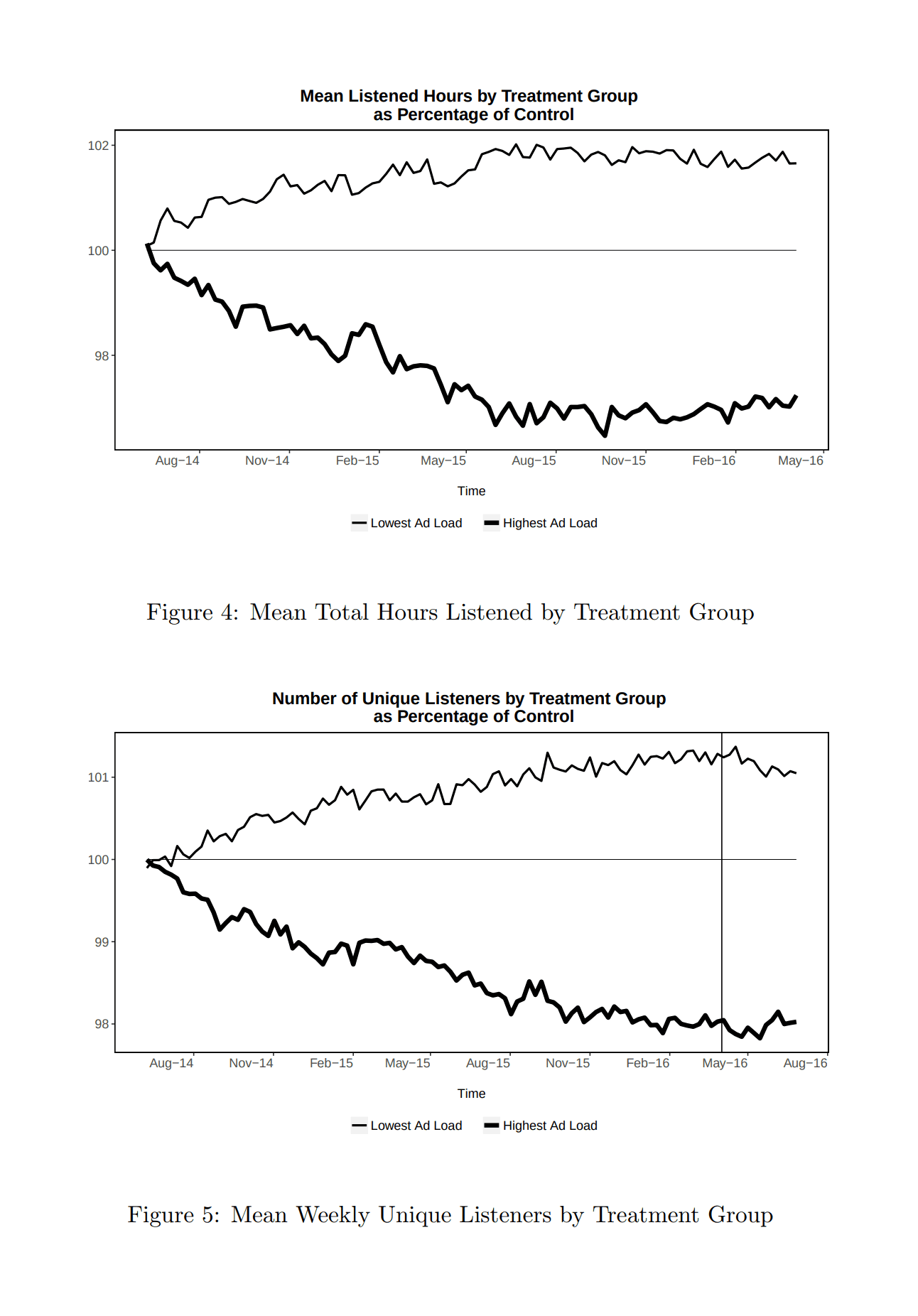
![Miroglio et al 2018, benefits to Firefox users from adblockers: “Figure 3: Estimates & 95% CI for B2, the change in log-transformed engagement due to installing add-ons [adblockers]”; “Table 5: Estimated relative changes in engagement due to installing add-ons compared to control group (exp(B2) − 1)”](/doc/economics/advertising/adblock/2018-miroglio-figure3table5-adblockerbrowseruse.png)

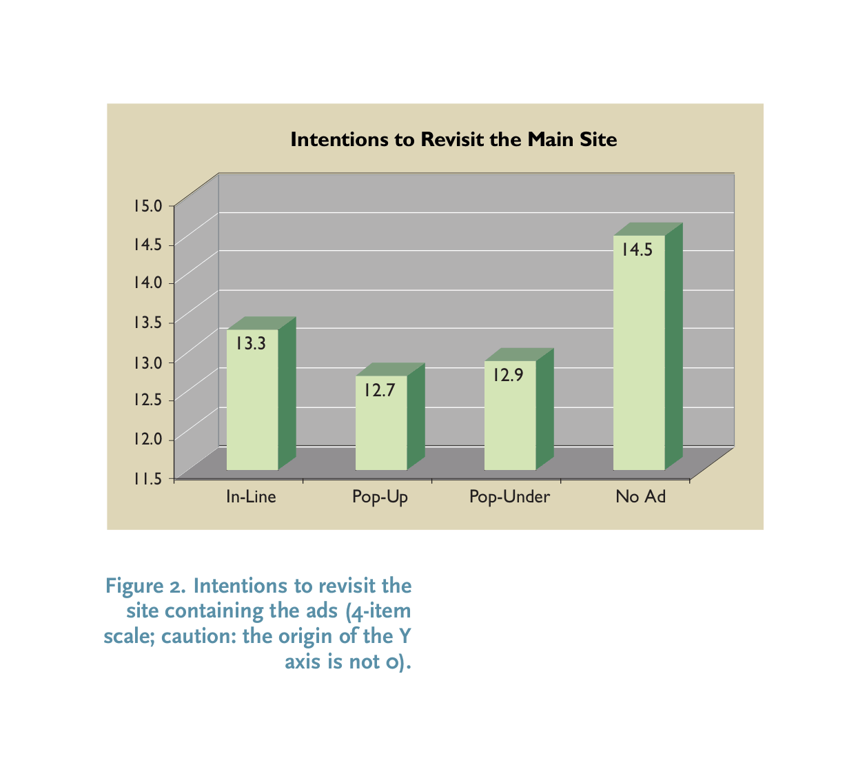
![Hohnhold et al 201511ya, benefit from 50% ad reduction on mobile over 2 month rollout of 10% users each: “Figure 6: ∆CTR [CTR = Clicks/Ad, term 5] time series for different user cohorts in the launch. (The launch was staggered by weekly cohort.)”](/doc/economics/advertising/2015-hohnhold-figure6-ctrratepostadreduction.png)


