Introducing a tool for interacting with generative models

Nolan Kent

Oct 27, 2019·17 min read

1.1: Preface

This is a technical blog about a project I worked on using Generative Adversarial Networks. As this was a personal project, I played around with an anime dataset that I wouldn’t normally use in a professional environment. Here’s a link to the dataset along with a detailed write-up about models that use the dataset:

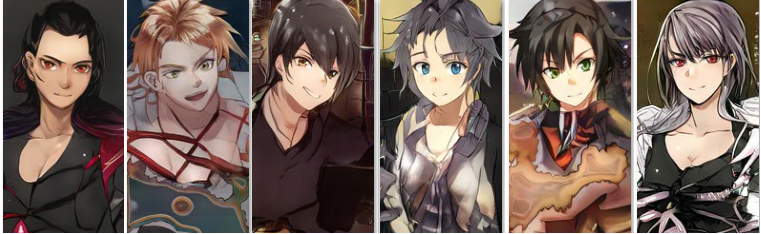
Most of the work I did was purely for learning purposes, but some of the more interesting results I ended up with were mouth animations for rectangular portraits:

I’ll go into the technical details of what I did and some of the lessons I learned. Part of the project was a tool to make interacting with and learning about generative adversarial networks easier, but at this point it is not user friendly. If I continue with this project one of my goals will be to publish a version of that tool that anyone can immediately start using to create animations like Figure 2, but right now it is primarily a tool for research:

I’ve found that incorporating experimental code into a tool like this instead of working with a jupyter notebook makes it much easier to repeat experiments with different settings. Some concepts only really stick through repetition, so without the tool I feel like I would have missed out on several of the insights mentioned in the blog. If you’re just interested example animations and not the technical details, you can skip to the Results: Animation section.

One of the main problems with personal projects is that they only involve a single perspective. My goal for this blog is to get other’s perspective on the topic, detail my experience working on the project and receive constructive criticism/corrections.

1.2: Introduction and Results Summary

I’ve been in the habit of regularly reimplementing papers on generative models for a couple years, so I started this project around the time the StyleGAN paper was published and have been working on it on and off since then. It includes 3 main parts:

1. A reimplementation of StyleGAN with some tweaks

2. Models trained using that implementation

3. A tool used to visualize and interact with the models

I started out reimplementing StyleGAN as a learning exercise, and because at the time the official code was not available. The results were so much better than the other models I worked with that I wanted to go more in depth. One application of generative models that I’m excited about is automatic asset creation for video games. StyleGAN is the first model I’ve implemented that had results that would acceptable to me in a video game, so my initial step was to try and make a game engine such as Unity load the model. To do this I made a .NET DLL which could interact with the model and theoretically be imported into Unity. To test the DLL I created a harness to interact with it. I ended up adding more and more features to the harness as I thought of them, until it became one of the biggest parts of the project. Here’s the overall architecture:

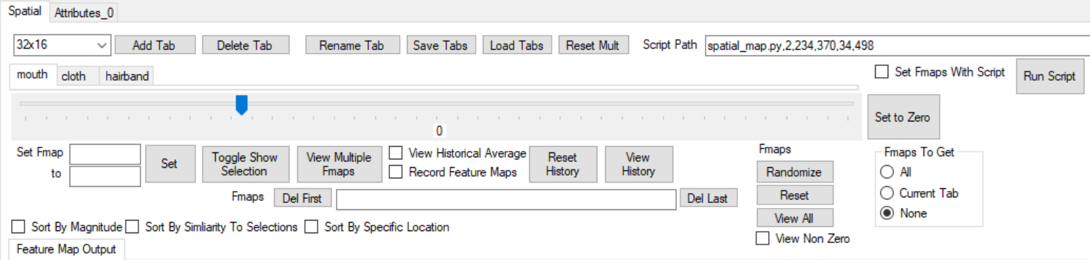
I’m a fan of using tools to visualize and interact with digital objects that might otherwise be opaque (such as malware and deep learning models), so one feature I added was visualization of feature maps (Figure 5) and the ability to modify them. Observing where feature maps at various layers are most active across different images helped me understand what the model was doing, and made it simple to automatically locate some facial features. When it came to modification, I noticed that adding or subtracting values from feature maps in specific locations could be used to make meaningful changes — for example opening and closing a mouth (Figure 2). Combined with automatic facial feature detection, this can be used to make consistent, meaningful modifications in all images generated without needing labels (Figure 9,10).

To summarize: a feature uses feature maps to modify facial features.

Here’s how the rest of the blog is structured:

• Applications of generative models
• Animations generated by the tool
• Brief discussion of the code
• Reimplementation details
• Discussion of the data
• Discussion of the training procedure

Applications

Overall, there are several applications that make me interested in generative models:

• Better procedural generation for game assets
• Making the creation of art easier and faster
• The fundamental potential of unsupervised learning combined with disentanglement of generative factors

Better procedural generation for game assets

I am excited about the possibility of generative models bringing procedural generation to the next level. As far as I’m aware, modern rules based procedural generation techniques cannot randomly create samples from highly complex distributions. For example, a subsection of a procedurally generated level can be mostly independent from the rest of the level and still be acceptable to a player. Randomly generating graphics such as character portraits is much more difficult, as good-looking images tend to reflect the real world which has so many inter-dependencies that each pixel needs to be considered in the context of every other pixel. Even stylized/drawn images need consistent lighting, anatomy, textures, perspective, style, etc. in order to look good. This also applies to automatically generating audio, dialog, animations, and story-lines. Generative models are currently the best way I’m aware of to reliably create samples from such complicated distributions.

Making the creation of art easier and faster

In the context of generative models, interactive tools also have the potential to allow laypersons to create images that would otherwise require an experienced artist, or allow artists to speed up the more routine parts of their work. I don’t think generative models are going to remove the need for creative artists any time soon, as generative models (along with most machine learning models) focus on modeling a specific distribution. This makes creating high quality images that are different from any samples in the training distribution (creative images) difficult. Tools like the one used in this blog that allow humans to add custom alterations can help to produce more unique images however, especially if the model has learned some fundamental graphical concepts such as lighting and perspective.

The fundamental potential of unsupervised learning combined with disentanglement of generative factors

As unlabeled data vastly outnumbers labeled data and deep learning is extremely data hungry, I think unsupervised/semi-supervised learning has the potential gradually replace supervised methods in the coming years. Some approaches to deep generative models in particular have been made to disentangle the factors of variation in a dataset: see Figure 7, 8 for examples of how StyleGAN can do this (at least partially). There isn’t actually an agreed upon formal definition of disentangment, and my understanding is that there is limited experimental evidence that it is useful for downstream tasks. However, working with GANs has made me optimistic that it will be useful. While the generator can not classically produce internal representations for images it did not generate, there are several other types of generative models that can compete with GANs in visual quality and may be better suited for downstream tasks.

Results: Animations

The best model I was able to train was on an anime dataset (https://gwern.net/Danbooru2018). I’ll go into the advantages and disadvantages of that in the data section, one of the main disadvantages being a lack of diversity: it is harder to produce male images. All of the examples below were generated with the tool. I originally created images like these in a jupyter notebook, but having a dedicated tool sped things up significantly and gave me a different perspective into how the model works. The images below are roughly ordered by how complicated it is to make them: Figures 7/8 require more work than Figure 6, and without a tool Figures 9/10 would have been harder to create than Figures 7/8.

Figure 6 is an example of interpolation between the intermediate latent variables of several images. A cool result that GANs can achieve is ensuring the interpolated images have quality similar to the end points.

Figure 7 is an example of modifying an image by locating a vector in the intermediate latent space with a certain meaning (in this case hair or eye color) and moving in that direction. For example, the vector for black hair can be found by taking many images of faces with black hair and averaging their latent values, and subtracting the result from the average of all other images. I’ll discuss this more in the Training/Postprocessing section.

Figure 8 shows the same concept used to generate Figure 7 when applied to the attribute ‘mouth open’. This works to some extent, but the attribute is not perfectly disentangled: changes can be seen in every part of the image, not just at the mouth. Common sense tells us that a person can move their mouth without significantly changing much else. A simple hack could be to paste the animated mouth on an otherwise static image, but this won’t work in cases where changing the ‘mouth open’ vector also changes skin tone or image style.

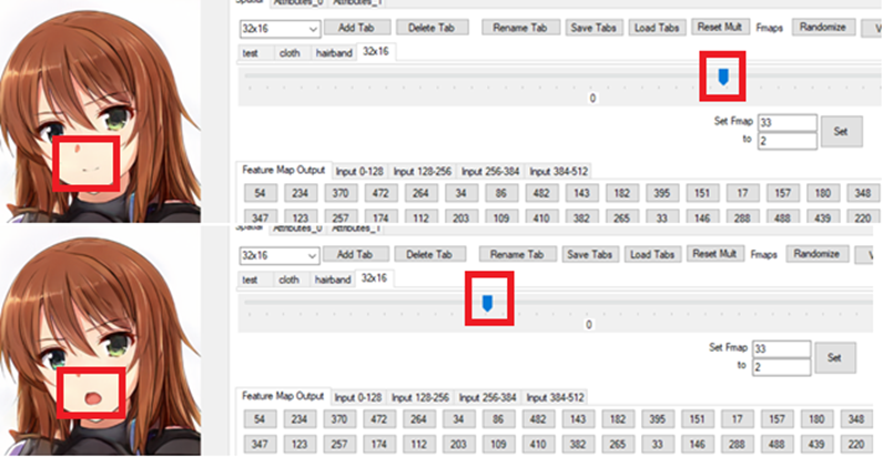
Figure 9 shows an example of modifying a specific feature map at a spatial location close to the character’s mouth to produce a talking (or chewing) animation that does not cause global changes. With a little bit of manual work, the feature map(s) that need to be modified to produce this change can be found without needing more than a couple examples of labeled data. All of this can be done through the tool. The process is inspired by how the DCGAN paper demonstrated window deletion by modifying feature maps. The modifications are simple additions or subtractions to local areas of specific feature maps. I’ll show how this can be done with the tool in a future blog.

Figure 10 shows the same thing as Figure 9, except applied to the presence/absence of a hairband. This technique can be applied to many different attributes.

Results: Code

Given my limited free time and that my primary goal was learning, I deprioritized a few aspects that are important to most projects:

• Planning/design: I started with as little planning as possible and added features/changes as I thought of them
• UI design: I used a greedy approach to adding features as I thought of them.
• Code style: I did not go into the project with the intent for others to read the code, instead my goal was to get results as fast as possible. With a malware reverse engineering background, I’m not particularly bothered by needing to debug low quality code myself. Moving fast worked well for the tool, but I go much slower for implementing the deep learning models as mistakes can be hard to catch and debug. The code quality is far from what would be acceptable for professional projects.

With these disclaimers out of the way, here’re the gitub links. They are under active development so there may be breaking bugs in some commits:

StyleGAN reimplementation:

Tool:

1.3: Implementation Details

In this section I’ll go into the technical details of what I did to reimplement StyleGAN and train a model with it

StyleGAN reimplementation

I started reimplementing StyleGAN shortly after the paper came out, which was a few months before the official code was released. I’ll discuss some of the challenges I encountered and approaches I took in this section, which assumes familiarity with the StyleGAN paper and TensorFlow.

StyleGAN is based on PGGAN, which I had already reimplemented. These models use ‘progressive growing’, where the discriminator and generator grow during training to handle higher and higher resolutions. Growing a model is somewhat uncommon — all other models I’ve implemented have never needed to change their architecture during training. Fortunately, TensorFlow has some convenient functions, such as the ability to load saved weights for only parts of a model and randomly initialize the rest. This is also used in transfer learning.

I really like the TensorFlow 2.0 style of creating models as classes that inherit from tf.keras.Model. I created most of the layers, the generator, the discriminator, and the mapping network this way. I also tried to make it an option to switch between eager execution and traditional graph-based execution. Eager execution allows for much easier debugging, which I view as a way to better understand a program (a common technique in malware analysis). Unfortunately, at the time eager execution seemed to be significantly slower than running in graph mode, so eventually I stopped keeping that functionality up to date. One of the nice things about using tf.keras.Model is that it works for both eager and graph mode, so theoretically it should not be too difficult to get eager working again. In the mean time I’ve just used the tfdebug command line interface and TensorBoard which I’m fairly comfortable with at this point.

StyleGAN has a few important differences from PGGAN. There’s the titular method of supplying the image-specific latent data as a style (non-spatial attribute) to the feature maps while using an “adaptive instance normalization” operation. Conceptually this is straight forward to implement as detailed in the paper, but my choice to use tf.nn.moments to calculate mean and variance did not work as well as the official implementation’s version which calculated these values with lower level operations. My first guess was that this was due to numerical issues, which was not something I felt like debugging at the time so I did not end up looking into it more. I’m usually happy to look deeper into issues like this as they’re obvious chances to learn more, but as this project is a hobby I have to prioritize to make the best use of my time.

StyleGAN also uses an intermediate latent space which hypothetically (with some empirical evidence presented in the paper) promotes disentanglement by adding flexibility and dependencies to the range of latent values. For example, if we assume a population where men never have long hair, a latent vector that corresponds to hair length should never be in the ‘long hair’ region when another latent that corresponds to gender is in the ‘male’ region. If the latent vectors are independent, which is what happens without the mapping network, and we end up sampling ‘long hair’ alongside ‘male’, the generator will have to create an image that is either not male or has short hair in order to fool the discriminator. This means even if the hair length latent is in the ‘long hair’ region, we may end up creating an image with short hair when other latent values are in normal parts of their range. Note that some definitions of disentanglement require axis-alignment (modifying a single latent value results in a meaningful change), while my understanding is that the mapping network of StyleGAN encourages the intermediate latent space to be a rotation of axis-aligned disentanglement (modifying a vector of latent values results in a meaningful change).

In my opinion the use of intermediate latent values is just as interesting as incorporating information into the network via styles. It is also simple to implement. When I refer to latent value throughout this blog series I will be referring to the intermediate latent value unless otherwise specified.

It is annoyingly common for what initially looks like a minor detail in a paper to turn out to be the most difficult part to implement. This was the case for StyleGAN — one difference between StyleGAN and PGGAN is the use of bilinear upsampling (and downsampling) and of R1 regularization (a gradient penalty on the discriminator). Both of these are simple to implement individually, however when I tried to combine them it turned out that TensorFlow did not have a way to compute the second derivative of the tf.nn.depthwise_conv2d operation. Depth-wise convolutions are used to apply a filter individually to each channel. This is not normally needed in convolutional neural networks because (outside some CNNs meant for mobile devices) each filter connects to all channels in the previous layer. The blur filter that is commonly used to implement bilinear interpolation operates on one feature map at a time, so it requires a depthwise convolution. Without a second derivative implemented, I couldn’t compute the R1 penalty which requires taking the gradient of a gradient. At the time I didn’t know enough about automatic differentiation to easily implement the second derivative myself. I spent some time trying to get a better understanding, however at that point I had everything finished except for this part, and a short time later the official code was released. The team at Nvidia solved the problem nicely using two tf.custom_gradient functions in the blur filter.

I made several experimental tweaks to StyleGAN with varying degrees of success.

1. I tested out rectangular images by changing the initial resolution to 8x4 and growing from there

2. I tried conditioning StyleGAN using ACGAN and cGan with Projection Discriminator

Rectangular images worked well. Conditioning on labels with ACGAN and cGan did not. This may have been due to my hyperparameter selections, but generally the results were worse than training without conditioning and then finding vectors in latent space that corresponded to meaningful features (discussed in Training/Postprocessing section).

Data

The FFHQ dataset — a collection of 70,000 high resolution images — was released alongside the StyleGAN paper. To get closer to the goal of generating entire people, I tried modifying the data extraction script supplied by Nvidia to extract images with an 8:4 (h:w) aspect ratio. In addition to extracting the face, this extracted the same amount of data from below the face. Doubling both the height and the width would require accounting for 4x the input dimensions, but just doubling the height requires 2x the dimensions. Data below a person’s face should also have less variance (variance mostly comes from different clothing) than background data, and not capturing background data means the network does not need to dedicate capacity to data that isn’t part of the person.

Unfortunately, only 20,000 of the 70,000 images in the FFHQ dataset had enough data below the person’s face to create images with the desired aspect ratio. As can be seen in Figure 11, I was not able to get particularly high quality results with this small dataset, but there may be ways to improve the quality (such as expanding the criteria for including an image).

I am also interested in the ability of GANs to perform on stylized drawings, and I saw that https://gwern.net/Danbooru2018 had recently been released. This dataset has a large number of high resolution images with very rich tag data. It does have some potential downsides, such as a disproportionately small number of male images which significantly reduces the quality of images in that class (Figure 12). The male images in this figure were the highest quality images cherry-picked out of around 1000 total images generated. I do think there is a lot of potential for improvement here, particularly using the truncation trick around the average male image.

The dataset also contains a significant portion of NSFW images, though I think one potential use of generative models is automatically modifying media to make it more suitable for different audiences.

To select candidate images to include, I was able to take advantage of metadata including ‘favorites’ (how many people favorited an image), resolution, tags, and creation date. To reduce variance and increase quality, I excluded images with few favorites and images that were created more than 6 years ago. I also only kept images with a resolution of at least 512x256 (HxW), my target resolution for the model. Finally, I filtered out images with tags that would increase variance in a portrait-style dataset, such as ‘lying_down’ and ‘from_side’, or that implied very NSFW images.

To generate the data I used a combination of the following two tools which I modified to extract the images of the desired aspect ratio:

These tools did not always extract images correctly, so I used illustration2vec to filter the result, as images where a person could not be detected were likely bad.

I also created a tool that would display a large grid of images from which I could manually delete bad images quickly, but this became too time consuming for datasets above 30,000 images. I ended up with several different datasets by including images of various qualities and tags which ranged from 40,000 to 160,000 images. All of these resulted in much better models than the 20,000 image FFHQ dataset I built.

Training/Postprocessing

I trained the model using as many as 80 epochs per resolution, which breaks down to 40 epochs for the PGGAN transition phase and 40 epochs for the stabilization phase. For the 160,000 image dataset this took over a month, and was probably overkill. I used Horovod to distribute training across two Nvidia Titan RTX graphics cards, which allowed large batch sizes in the early steps, and kept me from needing to ever go below 16 samples per batch.

To gather attributes I generated hundreds of thousands of images and scanned them with illustration2vec to get attribute estimates. For each attribute with more than 1000 corresponding images, I averaged the latent values together and subtracted them from the overall average image. This creates a vector that, when added to a latent, should promote the expression of the desired attribute. While this worked pretty well (which I interpret as further evidence the mapping network disentangles attributes), I’m interested in improving the process, potentially by using techniques described in https://arxiv.org/abs/1907.10786. In some cases I tried to manually disentangle correlated attributes: for example if blonde hair is correlated with blue eyes, subtracting a vector that corresponds to blue eyes from the blonde hair vector may help a bit. I then exported these attributes vectors into a csv file that could be loaded by the tool.

Conclusion/Misc Notes

I’ve gained a lot of experience by trying to reimplement papers that rely on fundamentals I don’t understand and then learning those fundamentals with a clear context for how they are used. The process feels a lot like backpropagation, and means I’ve spent 30+ hours trying to fully understand a single paper early on. This is the first time I’ve tried creating a tool to enhance that understanding, and I think it may become a standard strategy for me going forward.

I believe visual tools are a great way to improve understanding of a topic. Coming from a malware analyst background, tools like Hiew were essential in shaping how I understand malware, even though it was not initially intuitive how visual analysis can be helpful for windows executables. Given the bandwidth and processing power available to the human visual system, my hypothesis is that we can quickly gain a lot of insight from most data with spatially local structures when represented as an image. This is also the type of data that convolutional neural networks seem to work well with (not too surprising given their biological inspiration). The concept also applies to convolutional networks themselves, which is one part of why I worked on this project: hopefully visualizing the feature maps of convolutional neural networks might help me understand them better.

In the next part of this blog series I go into more detail about the tool and how it can be used to create animations. I also share a compiled version of the tool and a trained model to interact with, as the process to do that with just the source code is complicated at the moment.