To better understand the secular changes in the Black/White cognitive ability gap in the US, I plotted the standardized differences from our nearly 100 year review against row number. As samples were chronologically ordered, this provides a initial look at the relation between the magnitude of the gap and time.

The graph shows a midway increase and then a slight decline. This analysis, though, is confounded by interactions between age, representativeness of scores, and the magnitude of the difference. To better explore the issue, I removed clearly unrepresentative and redundant samples, separated scores into three age cohorts — below 6 (in red), 6-18 (in green), and above 18 (in blue) — and then plotted the ds by cohort by year/ estimated year. For standardized differences that were based on reviews, the average of the years covered in the review was used. For example, sample 5a represents a summary of scores of studies which were conducted between 1921 and 1944. For this point an average date of 1933 was used. The results are shown below:
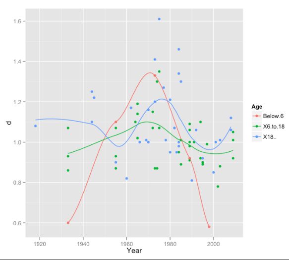
Again, we see an increase in the difference midway and then a slight decline. This analysis is possibly confounded by an interaction between sample type and standardized difference. We end up comparing aggregated scores by decade but scores in different decades might be heavily influenced by the types of studies done at a particular time. To deal with this problem, I identified relatively comparable samples based on age, the test given, and the representativity of the sample and look at the changes in the magnitude of the gap between these similar samples. The results are shown below:

Here we see a decline in the magnitude of the gap since the 1960s and 1970s. The rate of change is .005 SD/ year. This magnitude is quite similar to that reported by Sackett and Shen (2008) based on their regression model of changes in math and reading ds with age taken into account:

Projecting backwards this gives us a d of 1.45 in the 1920s which is inconsistent with the totality of the evidence on the magnitude of the gap at that time. The average pre-60s gap seems to have been about 1 to 1.2 SD or about what it was in the 1960s. The inconsistency between the projected magnitude of the gap in the 1920s based on the rate of change since and the magnitude of the gap based on the totality of the evidence suggests that either the pre-60s data underestimates the true magnitude of the gap at that time, which is possible since none of the samples before the late 1950s and early 1960s were nationally representative or that only since the 1960s has the gap noticeably narrowed, which is possible since most of the social policies introduced to eliminate the gap (e.g., positive discrimination for Blacks) were introduced after the ’60s. To address the first possibility, I reviewed the pre-60s data as thoroughly as could be done. Not infrequently, I found that the reported ds in narrative summaries were inflated relative to the ds in the original studies. For example, Jensen (1998) gives a WWII AGCT d of 1.25 and Gottfredson gives a WWI composite d of 1.17 when for both the correct values were somewhat less. Generally, the ds as I summarized them accurately capture the magnitude of the gap as reported in the literature.
Nonetheless it could be that the worst off Blacks were systematically underrepresented in the early studies. This possibility has to be balanced against the equally likely possibility that early studies were psychometrically (or culturally) biased against Blacks, thus inflating the mean between race difference. Since the 1980s, psychologists have put considerable effort into detecting and eliminated cultural bias. This was not the case in the early 1900s as critics of IQ testing have had great fun pointing out. These critics were probably not incorrect insofar as discussion concerns testing in the early 1900s, when IQ and other cognitive tests were first being developed and utilized. The implications is that early estimates of the BW difference need to be understood as estimates of the magnitude of the latent ability gap plus probable error due to test bias which tended to inflate the gap minus probably error due to sampling bias which tended to deflate the gap. My feeling is that the two types of error canceled each other out to a large extent and so that the aggregated reported score differences approximated the true population differences at the times in question.
Whatever the case, the amount of narrowing of the difference is much less than others have argued. For example, Sean Reardon of Stanford University gives the following graph, which points to a narrowing of almost two-thirds (from 1.5 SD to 0.5 SD) between 1940 and 2001:
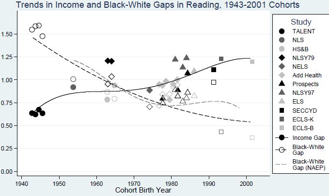
(Source: The Widening Academic Achievement Gap Between the Rich and the Poor:New Evidence and Possible Explanations)
Reardon’s analysis, of course, is deeply flawed by his failure to take into account both age effects and test content effects in addition to his dubious method of deriving early comparison points. As for the latter, he, for example, derives his early points, from the 1940s, from Charles Murray’s analysis of the 1976, 1986, and 1996 Woodcock–Johnson I to III standardizations. Of course, these samples were from the 70s, 80s, and 90s. To derive magnitudes of differences from the 40s, he projects back in time based on Murray’s birth cohort analysis. These differences, based on Full scale IQ — e.g., between 70 year old Blacks and Whites in the 90s who would have been 20 or so in the 40s — are then compared with the average Math and Reading differences between 5 to 7 year olds from the Early Childhood Longitudinal Study in the late 1990s (a study which showed a large effect of age on the magnitude of the math and reading gap — see: sample 48 — and also a large general knowledge gap at very young ages — see III, Chuck (2012c). His analysis, then, is confounded by the three problems and their interactions: (1) His method of deriving early points. (2) His comparison across measures. (3) And his comparison across ages.
As for the contemporaneous gap, I think that my 2012 estimate is fairly accurate:

Here “d subtest” refers to “Math and Reading” scores and “d composite” is the composite score calculated on the basis of these. We see that the gap increases with age, from 0.92 SD at ages 9 to 14 to 1.12 SD by adulthood. The mean gap is 1.02 SD.
Given this value that gap decreased by no more than 0.3 SD since the 1970s or by no more than 0.2 SD since the 1960s. And (probably) by no more than 0.2 since the 1920s. Now, this is curious because we would not expect this were the gap due to the family level inter-generational transference of IQ solely by way of the environment, as is often argued. The simplest family level inter-generational model is as follows:

By this model, the adult IQ gap of generation #1 is antecedent to the social outcome gaps of generation #1; this social outcome gap is antecedent to the childhood rearing environment gap of generation #2; and this childhood rearing environment gap is antecedent to the adult IQ gap of generation #2. And so on. One reason that this model is proposed is because it superficially fits the data: the IQ gaps of generation #1 do, in fact, statistically explain the social outcome gaps of generation #1 and the IQ and social outcome gaps of generation #1 largely statistically explains the IQ gaps of generation #2.
Now, since by adulthood the correlation between the totality of one’s shared environment which, in addition to genes, is what parents pass onto their children is, according to the behavioral genetic literature, no more than 0.4, one would expect that the gap would more than halve every generation if both populations had similar opportunities to realize their intellectual potential and if both populations had similar environments external to the rearing one. So, starting with an age 20-30 year old gap of 1.1 SD in 1960, the gap by 2010 should be about 0.15 SD in 2010 for the same age cohort, were differences, over the same time period, solely due to the environmental inter-generational transference of IQ at the family level. That is, shared environmental effects transmitted between families per se can not explain the inter-generational consistency of the difference. Blacks can not be said to be equivalent to the subpopulation of Whites who happen to have grandparents etc. who were reared in inferior environments because the effects of such shared environments wash out in two to three generations. In short, some other factor must be said to be conditioning the stability of the gap.
The above, of course, isn’t to say that population can’t pass on environmental effects over many generations. They can because populations also create the environments external to the family which allows individuals to realize their genetic potential differently relative to other family members. (In a parallel manner, populations can pass on genetic effects over many generations without the impact of these effects diminishing.) Such environmental population level effects, of course, are implausible causes of the differential in the US for a number of reasons. But that discussion is for another time. The point of importance here is that the race difference is unlike the within race difference due to family environmental advantages.

January 16, 2013 at 4:57 am
If you’re going to overlay scatterplots distinguished by color with curve fits, the curves ought to have the same color. Like many graphing problems, the answer is simple: use ggplot and it will do this for you. Also, it encourages you to use loess, which I think is good. plots here
library(reshape)
library(ggplot2)
bw <- read.csv("black-white-age-time.csv")
bwt <- melt(bw, id.vars="Year", variable_name="Age")
bwt2 <- rename(bwt, c(value="d"))
qplot(Year, d, color=Age, data=bwt2)+geom_smooth(se=F) # loess
qplot(Year, d, color=Age, data=bwt2)+geom_smooth(formula=y~poly(x,2), method=lm,se=F) # quadratic
Can I embed images?
January 16, 2013 at 4:59 am
(No, I can’t embed images.)