Self-experiment on whether screen-tinting software such as Redshift/f.lux affect sleep times and sleep quality; Redshift lets me sleep earlier but doesn’t improve sleep quality.
I ran a randomized experiment with a free program (Redshift) which reddens screens at night to avoid tampering with melatonin secretion & the sleep from 2012–2013, measuring sleep changes with my Zeo. With 533 days of data, the main result is that Redshift causes me to go to sleep half an hour earlier but otherwise does not improve sleep quality.
My earlier melatonin experiment found it helped me sleep. Melatonin secretion is also influenced by the color of light (some references can be found in my melatonin article), specifically blue light tends to suppress melatonin secretion while redder light does not affect it. (This makes sense: blue/white light is associated with the brightest part of the day, while reddish light is the color of sunsets.) Electronics and computer monitors frequently emit white or blue light. (The recent trend of bright blue LEDs is particularly deplorable in this regard.) Besides the plausible suggestion about melatonin, reddish light impairs night vision less and is easier to see under dim conditions: you may want a blazing white screen at noon so you can see something, but in a night setting, that is like staring for hours straight into a fluorescent light.
Hence, you would like to both dim your monitor and also shift the color temperature towards the cooler redder end of the spectrum with an utility like f.lux or Redshift.
But does it actually work? And does it work in addition to my usual melatonin supplementation of 1–1.5mg? An experiment is called for!
The suggested mechanism is through melatonin secretion. So we’d look at all the usual sleep metrics plus mood plus an additional one: what time I go to bed. One of the reasons I became interested in melatonin was as a way of getting myself to go to bed rather than stay up until 3 AM—a chemically enforced bedtime—and it seems plausible that if Redshift is reducing the interference of the computer monitor, it will make me stay up later (“but I don’t feel sleepy yet”).
Design
Power Calculation
The earlier melatonin experiment found somewhat weak effects with >100 days of data, and one would expect that actually consuming 1.5mg of melatonin would be a stronger intervention than simply shifting my laptop screen color. (What if I don’t use my laptop that night? What if I’m surrounded by white lights?) 30 days is probably too small, judging from the other experiments; 60 is more reasonable, but 90 feels more plausible.
It may be time to learn some more statistics, specifically how to do statistical power calculations for sample size determination. As I understand it, a power calculation is an equation balancing your sample size, the effect size, and the statistical-significance level (eg. the old p < 0.05); if you have 2, you can deduce the third. So if you already knew your sample size and your effect size, you could predict what statistical-significance your results would have. In this specific case, we can specify our statistical-significance at the usual level, and we can guess at the effect size, but we want to know what sample size we should have.
Let’s pin down the effect size: we expect any Redshift effect to be weaker than melatonin supplementation, and the most striking change in melatonin (the reduction in total sleep time by ~50 minutes) had an effect size of 0.37. As usual, R has a bunch of functions we can use. Stealing shamelessly from an R guide, and reusing the means and standard deviations from the melatonin experiment, we can begin asking questions like: “suppose I wanted a 90% chance of my experiment producing a solid result of p > 0.01 (not 0.05, so I can do multiple correction) if the Redshift data looks like the melatonin data and acts the same way?”
install.packages("pwr", depend = TRUE)
library(pwr)
pwr.t.test(d=(456.4783-407.5312)/131.4656,power=0.9,sig.level=0.01,type="paired",alternative="greater")
#
#      Paired t test power calculation
#
#               n = 96.63232
#               d = 0.3723187
#       sig.level = 0.01
#           power = 0.9
#     alternative = greater
#
#  NOTE: n is number of *pairs*
n is pairs of days, so each n is one day on, one day off; so it requires 194 days! Ouch, but OK, that was making some assumptions. What if we say the effect size was halved?
pwr.t.test(d=((456.4783-407.5312)/131.4656)/2,power=0.9,sig.level=0.01,type="paired",alternative="greater")
#
#      Paired t test power calculation
#
#               n = 378.3237
That’s much worse (as one should expect—the smaller an effect or desired p-value or chance you don’t have the power to observe it, the more data you need to see it). What if we weaken the power and significance level to 0.5 and 0.05 respectively?
pwr.t.test(d=((456.4783-407.5312)/131.4656)/2,power=0.5,sig.level=0.05,type="paired",alternative="greater")
#
#      Paired t test power calculation
#
#               n = 79.43655
#               d = 0.1861593
This is more reasonable, since n = 80 or 160 days will fit within the experiment but look at what it cost us: it’s now a coin-flip that the results will show anything, and they may not pass multiple correction either. But it’s also expensive to gain more certainty—if we halve that 50% chance of finding nothing, it doubles the number of pairs of days we need 79 → 157:
pwr.t.test(d=((456.4783-407.5312)/131.4656)/2,power=0.75,sig.level=0.05,type="paired",alternative="greater")
#
#      Paired t test power calculation
#
#               n = 156.5859
#               d = 0.1861593
Statistics is a harsh master. What if we solve the equation for a different variable, power or significance? Maybe I can handle 200 days, what would 100 pairs buy me in terms of power?
pwr.t.test(d=((456.4783-407.5312)/131.4656)/2,n=100,sig.level=0.05,type="paired",alternative="greater")
#
#      Paired t test power calculation
#
#               n = 100
#               d = 0.1861593
#       sig.level = 0.05
#           power = 0.5808219
Just 58%. (But at p = 0.01, n = 100 only buys me 31% power, so it could be worse!) At 120 pairs/240 days, I get 65% power, so it may all be doable. I guess it’ll depend on circumstances: ideally, a Redshift trial will involve no work on my part, so the real question becomes what quicker sleep experiments does it stop me from running and how long can I afford to run it? Would it painfully overlap with things like the lithium trial?
Speaking of the lithium trial, the plan is to run it for a year. What would 2 years of Redshift data buy me even at p = 0.01?
pwr.t.test(d=((456.4783-407.5312)/131.4656)/2,n=365,sig.level=0.01,type="paired",alternative="greater")
#
#      Paired t test power calculation
#
#               n = 365
#               d = 0.1861593
#       sig.level = 0.01
#           power = 0.8881948
Acceptable.
Experiment
How exactly to run it? I don’t expect any bleed-over from day to day, so we randomize on a per-day basis. Each day must either have Redshift running or not. Redshift is run from cron every 15 minutes: */15 * * * * redshift -o. (This is to deal with logouts, shutdowns, freezes etc, that might kill Redshift as a persistent daemon.) We’ll change the code to at the beginning of each day run:
@daily redshift -x; if ((RANDOM \% 2 < 1));
          then touch ~/.redshift; echo `date +"\%d \%b \%Y"`: on >> ~/redshift.log;
          else rm ~/.redshift; echo `date +"\%d \%b \%Y"`: off >> ~/redshift.log; fi
Then the Redshift call simply includes a check for the file’s existence:
*/15 * * * * if [ -f ~/.redshift ]; then redshift -o; fiNow we have completely automatic randomization and logging of the experiment. As long as I don’t screw things up by deleting either file or uninstalling Redshift, and I keep using my Zeo, all the data is gathered and labeled nicely until I finish the experiment and do the analysis. Non-blinded, or perhaps I should say quasi-blinded—I initially don’t know, but I can check the logs or file to see what that day was, and I will at some point in the night notice whether the monitor is reddened or not.
As it turned out, I received a proof that I was not noticing the randomization. 2013-01-11, due to Internet connectivity problems, I was idling on my computer and thought to myself that I hadn’t noticed Redshift turn my screen salmon-colored in a while, and I happened to idly try redshift -x (reset the screen to normal) and then redshift -o (immediately turn the screen red)—but neither did anything at all. Busy with other things, I set the anomaly aside until a few days later, I traced the problem to a package I had uninstalled back in 2012-09-25 because my system didn’t use it—which it did not, but this had the effect of removing another package which turned out to set the default video driver to the proper driver, and so removing it forced my system to a more primitive driver which apparently did not support Redshift functionality1! And I had not noticed for 3 solid months. This was a frustrating incident, but since it took me so long to notice, I am going to keep the 3 months’ data and keep them in the ‘off’ category—this is not nearly as good as if those 3 months had varied (since now the ‘on’ category will be underpopulated), but it seems better than just deleting them all.
So to recap: the experiment is 100+ days with Redshift randomized on or off by a shell script, affecting the usual sleep metrics plus time of bed. The expectation is that lack of Redshift will produce a weak negative effect: increasing awakenings & time awake & light sleep, increasing overall sleep time, and also pushing back bedtime.
VoI
Like the modafinil day trial, this is another value-less experiment justified by its intrinsic interest. I expect the results will confirm what I believe: that red-tinting my laptop screen will result in less damage to my sleep by not forcing lower melatonin levels with blue light. The only outcome that might change my decisions is if the use of Redshift actually worsens my sleep, but I regard this as highly unlikely. It is cheap to run as it is piggybacking on other experiments, and all the randomizing & data recording is being handled by 2 simple shell scripts.
Data
The experiment ran from 2012-05-11 to 2013-11-04, including the unfortunate January 2013 period, with n = 533 days. I stopped it at that point, having reached the 100+ goal and since I saw no point in continuing to damage my sleep patterns to gain more data.
Analysis
Preprocessing:
redshift <- read.csv("https://gwern.net/doc/zeo/2012-2013-gwern-zeo-redshift.csv")
redshift <- subset(redshift, select=c(Start.of.Night, Time.to.Z, Time.in.Wake, Awakenings,
                                      Time.in.REM, Time.in.Light, Time.in.Deep, Total.Z, ZQ,
                                      Morning.Feel, Redshift, Date))
redshift$Date <- as.Date(redshift$Date, format="%F")

redshift$Start.of.Night <- sapply(strsplit(as.character(redshift$Start.of.Night), " "), function(x) { x[2] })
## Parse string timestamps to convert "06:45" to 24300:
interval <- function(x) { if (!is.na(x)) { if (grepl(" s",x)) as.integer(sub(" s","",x))
                                           else { y <- unlist(strsplit(x, ":")); as.integer(y[[1]])*60 + as.integer(y[[2]]); }
                                         }
                          else NA
                        }
redshift$Start.of.Night <- sapply(redshift$Start.of.Night, interval)
## Correct for the switch to new unencrypted firmware in March 2013;
redshift[(as.Date(redshift$Date) >= as.Date("2013-03-11")),]$Start.of.Night <-
  (redshift[(as.Date(redshift$Date) >= as.Date("2013-03-11")),]$Start.of.Night + 900) %% (24*60)

## after midnight (24*60=1440), Start.of.Night wraps around to 0, which obscures any trends,
## so we'll map anything before 7AM to time+1440
redshift[redshift$Start.of.Night<420 & !is.na(redshift$Start.of.Night),]$Start.of.Night <-
 (redshift[redshift$Start.of.Night<420 & !is.na(redshift$Start.of.Night),]$Start.of.Night + (24*60))
Descriptive:
library(skimr)
skim(redshift)
# Skim summary statistics
#  n obs: 533
#  n variables: 12
#
# ── Variable type:Date ───────────────────────────────────────────────────────────────────────────────────────────────────────────────────────────────────────────────
#  variable missing complete   n        min        max     median n_unique
#      Date       0      533 533 2012-05-11 2013-11-04 2013-02-11      530
#
# ── Variable type:factor ─────────────────────────────────────────────────────────────────────────────────────────────────────────────────────────────────────────────
#  variable missing complete   n n_unique                top_counts ordered
#  Redshift       0      533 533        2  FA: 313,  TR: 220, NA: 0   FALSE
#
# ── Variable type:integer ────────────────────────────────────────────────────────────────────────────────────────────────────────────────────────────────────────────
#       variable missing complete   n   mean    sd p0    p25 p50    p75 p100     hist
#     Awakenings      17      516 533   7     2.92  0   5      7   9      18 ▁▃▆▇▂▁▁▁
#   Morning.Feel      20      513 533   2.72  0.84  0   2      3   3       4 ▁▁▁▅▁▇▁▂
#   Time.in.Deep      17      516 533  62.37 12.07  0  56     63  70      98 ▁▁▁▂▆▇▂▁
#  Time.in.Light      17      516 533 284.39 43.24  0 267    290 308     411 ▁▁▁▁▂▇▃▁
#    Time.in.REM      17      516 533 166.85 30.99  0 150    172 186     235 ▁▁▁▁▃▇▆▂
#   Time.in.Wake      17      516 533  22.45 19.06  0  12     19  28     276 ▇▁▁▁▁▁▁▁
#      Time.to.Z      17      516 533  23.92 13.08  0  16.75  22  30     135 ▃▇▂▁▁▁▁▁
#        Total.Z      17      516 533 513.1  71.97  0 491    523 553.25  695 ▁▁▁▁▁▆▇▁
#             ZQ      17      516 533  92.11 13.54  0  88     94 100     123 ▁▁▁▁▁▆▇▁
#
# ── Variable type:numeric ────────────────────────────────────────────────────────────────────────────────────────────────────────────────────────────────────────────
#        variable missing complete   n    mean    sd   p0  p25  p50  p75 p100     hist
#  Start.of.Night      17      516 533 1444.06 49.72 1020 1415 1445 1475 1660 ▁▁▁▁▅▇▁▁

## Correlation matrix:
## Drop date; convert Redshift boolean to 0/1; use all non-missing pairwise observations; round
redshiftInteger<- cbind(redshift[,-(11:12)], Redshift=as.integer(redshift$Redshift))
round(digits=2, cor(redshiftInteger, use="complete.obs"))
#                Start.of.Night Time.to.Z Time.in.Wake Awakenings Time.in.REM Time.in.Light Time.in.Deep Total.Z    ZQ Morning.Feel Redshift
# Start.of.Night           1.00
# Time.to.Z                0.19      1.00
# Time.in.Wake             0.05      0.23         1.00
# Awakenings               0.22      0.17         0.36       1.00
# Time.in.REM              0.08     -0.09        -0.14       0.29        1.00
# Time.in.Light            0.05     -0.08        -0.18       0.23        0.56          1.00
# Time.in.Deep             0.08     -0.08        -0.03       0.15        0.40          0.30         1.00
# Total.Z                  0.08     -0.10        -0.17       0.29        0.84          0.90         0.53    1.00
# ZQ                       0.06     -0.15        -0.31       0.13        0.84          0.81         0.64    0.97  1.00
# Morning.Feel             0.04     -0.22        -0.24      -0.01        0.38          0.37         0.27    0.44  0.46         1.00
# Redshift                -0.19     -0.07         0.03      -0.04       -0.01         -0.03        -0.14   -0.05 -0.07         0.04     1.00

library(ggplot2)
qplot(Date, Start.of.Night, color=Redshift, data=redshift) +
  coord_cartesian(ylim=c(1340,1550)) + stat_smooth() +
  ## Reverse logical color coding, to show that red-tinted screens = earlier bedtime:
  scale_color_manual(values=c("blue", "red"))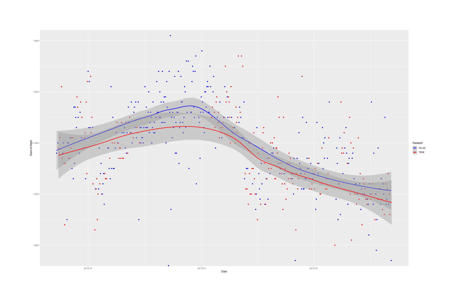
Analysis:
l <- lm(cbind(Start.of.Night, Time.to.Z, Time.in.Wake, Awakenings, Time.in.REM, Time.in.Light,
              Time.in.Deep, Total.Z, ZQ, Morning.Feel) ~ Redshift, data=redshift)
summary(manova(l))
##            Df     Pillai approx F num Df den Df     Pr(>F)
## Redshift    1 0.07276182 3.939272     10    502 3.4702e-05
## Residuals 511
summary(l)
## Response Start.of.Night :
## ...Coefficients:
##                 Estimate Std. Error   t value   Pr(>|t|)
## (Intercept)   1452.03333    2.82465 514.05791 < 2.22e-16
## Redshift TRUE  -18.98169    4.38363  -4.33014 1.7941e-05
##
## Response Time.to.Z :
## ...Coefficients:
##               Estimate Std. Error  t value Pr(>|t|)
## (Intercept)   24.72333    0.75497 32.74743  < 2e-16
## Redshift TRUE -1.87826    1.17165 -1.60309  0.10953
##
## Response Time.in.Wake :
## ...Coefficients:
##               Estimate Std. Error  t value Pr(>|t|)
## (Intercept)   22.13333    1.10078 20.10704   <2e-16
## Redshift TRUE  1.02160    1.70831  0.59801   0.5501
##
## Response Awakenings :
## ...Coefficients:
##                Estimate Std. Error  t value Pr(>|t|)
## (Intercept)    7.133333   0.167251 42.65047  < 2e-16
## Redshift TRUE -0.260094   0.259560 -1.00206  0.31679
##
## Response Time.in.REM :
## ...Coefficients:
##                 Estimate Std. Error  t value Pr(>|t|)
## (Intercept)   167.713333   1.732029 96.83056  < 2e-16
## Redshift TRUE  -0.849484   2.687968 -0.31603  0.75211
##
## Response Time.in.Light :
## ...Coefficients:
##                Estimate Std. Error   t value Pr(>|t|)
## (Intercept)   286.20667    2.43718 117.43332  < 2e-16
## Redshift TRUE  -2.98601    3.78231  -0.78947  0.43021
##
## Response Time.in.Deep :
## ...Coefficients:
##                Estimate Std. Error t value   Pr(>|t|)
## (Intercept)   63.863333   0.686927 92.9696 < 2.22e-16
## Redshift TRUE -3.436103   1.066055 -3.2232  0.0013486
##
## Response Total.Z :
## ...Coefficients:
##                Estimate Std. Error   t value Pr(>|t|)
## (Intercept)   517.29333    4.00740 129.08467  < 2e-16
## Redshift TRUE  -7.30272    6.21915  -1.17423  0.24085
##
## Response ZQ :
## ...Coefficients:
##                Estimate Std. Error   t value Pr(>|t|)
## (Intercept)   93.053333   0.758674 122.65253  < 2e-16
## Redshift TRUE -1.799812   1.177401  -1.52863  0.12697
##
## Response Morning.Feel :
## ...Coefficients:
##                Estimate Std. Error  t value Pr(>|t|)
## (Intercept)   2.6933333  0.0485974 55.42136   <2e-16
## Redshift TRUE 0.0719249  0.0754192  0.95367   0.3407
wilcox.test(Start.of.Night ~ Redshift, conf.int=TRUE, data=redshift)
#
#    Wilcoxon rank sum test with continuity correction
#
# data:  Start.of.Night by Redshift
# W = 39789, p-value = 6.40869e-06
# alternative hypothesis: true location shift is not equal to 0
# 95% confidence interval:
#   9.9999821 24.9999131
# sample estimates:
# difference in location
#             15.0000618
To summarize:
|
Measurement |
Effect |
Units |
Goodness |
p |
|---|---|---|---|---|
|
Start of Night |
−18.98 |
minutes |
+ |
<0.001 |
|
Time to Z |
−1.88 |
minutes |
+ |
0.11 |
|
Time Awake |
+1.02 |
minutes |
− |
0.55 |
|
Awakenings |
−0.26 |
count |
+ |
0.32 |
|
Time in REM −0.85 minut |
es − |
0. |
75 |
|
|
Time in Light |
−2.98 |
minutes |
+ |
0.43 |
|
Time in Deep |
−3.43 |
minutes |
− |
0.001 |
|
Total Sleep |
−7.3 |
minutes |
− |
0.24 |
|
ZQ |
−1.79 |
? (index) |
− |
0.13 |
|
Morning feel |
+0.07 |
1–5 scale |
+ |
0.34 |
Bayes
In December 2019, I attempted to re-analyze the data in a Bayesian model using brms, to model the correlations & take any temporal trends into account with spline term, fitting a model like this:
library(brms)
bz <- brm(cbind(Start.of.Night, Time.to.Z, Time.in.Wake, Awakenings, Time.in.REM, Time.in.Light,
              Time.in.Deep, Total.Z, ZQ, Morning.Feel) ~ Redshift + s(as.integer(Date)), chains=30,
              control = list(max_treedepth=13, adapt_delta=0.95),
              data=redshift)
bz
Unfortunately, it proved completely computationally intractable, yielding only a few effective samples after several hours of MCMC, and the usual fixes of tweaking the control parameter and adding semi-informative priors didn’t help at all. It’s possible that the occasional outliers in Start.of.Night screw it up, and I need to switch to a distribution better able to model outliers (eg. loosen the default normal/Gaussian to a Student’s t with family="student") or drop outlier days. If those don’t work, it may be that simply modeling them all like that is inappropriate: they all have different scales & distributions. brms doesn’t support full SEM modeling like blavaan, but it does support multivariate variables with differing distributions, I believe—it just requires a good deal more messing with the model definitions. Since fitting was so slow, I dropped my re-analysis there.
Conclusion
Redshift does influence my sleep.
One belief—that Redshift helped avoid bright light retarding the sleep cycle and enabling going to bed early—was borne: on Redshift days, I went to bed an average of 19 minutes earlier. (I had noticed this in my earliest Redshift usage in 2008 and noticed during the experiment that I seemed to be staying up pretty late some nights.) Since I value having a sleep schedule more like that of the rest of humanity and not sleeping past noon, this justifies keeping Redshift installed.
But I am also surprised at the lack of effect on the other aspects of sleep; I was sure Redshift would lead to improvements in waking and how I felt in the morning, if nothing else. Yet, while the exact effect tends to be better for the most important variables, the effect estimates are relatively trivial (less than a tenth increase in average morning feel? falling asleep 2 minutes faster?) and several are worse—I’m a bit baffled why deep sleep decreased, but it might be due to the lower total sleep.
So it seems Redshift is excellent for shifting my bedtime forward, but I can’t say it does much else.
External Links
-
The geeky details: I found an error line in the X logs which appeared only when I invoked Redshift; the driver was
fbdevand not the correctradeon, which mystified me further, until I read various bug reports and forum problems and wondered whyradeonwas not loading but the only non-fbdeverror message indicated that some driver calledatiwas failing to load instead. Then I read thatatiwas the default wrapper overradeon, but then I saw that the package was not installed, installed it, noticed it was pulling in as a dependency useless Mach64 drivers, and had a flash: perhaps I had uninstalled the useless Mach64 drivers, forcing the package providingatito be uninstalled too, permitted its uninstallation because I knew it was not the package providingradeon, which then caused theatiload to fail and to not then loadradeonbut X succeeding in loadingfbdevwhich does not support Redshift, leading to a permanent failure of all uses of Redshift. Phew! I was right.↩︎