Life Extension Cost-Benefits
Attempts at considering the profitability of life-extension interventions for healthy adults
We all want to live longer, but I find most discussions of available interventions unsatisfying because they tend to ignore any consideration of whether the intervention is too expensive (as the joke about veganism/caloric restriction goes, you may live longer but will you want to?), and be simultaneously too gullible (nutrition research; looking at any health parameter which improves) and too narrow-minded (I don’t care if an intervention has p > 0.05 if that still means a 90% probability of benefit).
What I would like to see is a practical guide, taking a decision theory perspective, which follows a procedure something like the following, in taking interventions which:
reduce “all-cause mortality”,
ACM is the end-point of choice for life-extension because it is both closest to what we care about (additional life) and it is the hardest of all end-points - it is difficult to cheat, miscount, or not notice, and by being simple, consistent, and unambiguous, avoids many failure modes such as subgroup hacking or dropping outliers or tweaking covariates (either a larger fraction of the controls are dead or not). It also can typically be extracted from most studies, even if they otherwise fail to report much of the data.
From a benefit point of view, average reduction in all-cause mortality is excellent for ignoring any zero-sum tradeoffs: it’s no good if reported benefits are only because the doctors writing up a trial kept slicing deaths by different categorizations of causes until they finally found a p < 0.05 or if the gains only appear by excluding some deaths as ‘irrelevant’ or if the gains in one cause of death comes at the expense of another cause (is it really helpful to avoid death by heart attack if the intervention just means you die of cancer instead?). For example, one primate study of caloric restriction found benefits only if it excluded a bunch of deaths in the CR group and defined them as not age-related, ignoring “monkeys who died while taking blood samples under anesthesia, from injuries or from infections, such as gastritis and endometriosis.” (Even in the followup paper several years later, the all-cause mortality reduction is much smaller than the “age-related” subcategory.) From a life-extension perspective, it is irrelevant if an intervention reduces some kinds of diseases while making one much more prone to dying from routine causes such as injuries or minor operations under anesthesia (especially since, in modern societies, one is guaranteed to be operated on at some point) - it either reduces all-cause mortality or it doesn’t.
as estimated in randomized trials,
Correlation is not causation and correlates only rarely turn out to be usefully causal. With aging, the situation is especially severe since aging is the exponential increase in mortality with time as all bodily systems gradually begin to fail; one cannot simply take a correlation of some chemical with aging or mortality and expect an intervention on it to have more than a minute chance of making a difference, since almost every chemical or substance or biomarker will change with age (eg. papers on magnesium levels often note that surprisingly, blood levels of magnesium don’t change substantially with age). Worse, over more than a century of concerted effort and tinkering with a bewildering variety of thousands of interventions from injecting embryos to consuming testicles (or crushing one’s own) to yogurt to yoga, it can safely be said that (almost?) all tried interventions have failed, and the prior odds are strongly against any new one.
on healthy adult human populations
Studies of interventions in the sick are also unhelpful, as (hopefully!) the benefits observed may come from their particular disorder being treated. Animal studies are also unhelpful as results cross-species are highly unreliable and model organisms may age in entirely different manner from humans, who are unusually long-lived as it is. One challenge for this criteria is studies done in elderly populations: because death rates are so high, they offer higher power to detect reductions in mortality; but because that death rate is pushed so high due to the aging process, they will tend to have many chronic conditions and diseases as well. Do we ignore studies recruiting from, for example, 70-90yos who all inherently have health problems? I would say it’s probably better to err on the side of inclusion here as long as subjects were not selected for any particular health problem.
for which there are enough trials to do a random-effects/multilevel model, so one can extract a posterior predictive interval of the benefit,
It’s important to include heterogeneity from population to population as part of the uncertainty. One of the subtleties often missed in dealing with modeling is that a 95% CI around a parameter is not a CI around the outcome or result.
letting one compare mortality reduction against intervention cost,
For making decisions, the costs of the intervention must be taken into account. A taxing exercise regimen may be proven to increase longevity, but is that of any value of the regimen takes away much more of your life than it gives back? It may be that no matter whether our certainty is 99% or 99.99% that it works, we would never choose to embark on that regimen. On the other hand, for a cheap enough intervention, we may be willing to accept substantially lower probability: baby aspirin, for example, costs $7 & <10 seconds each morning / <60 minutes a year and we might be willing to use it if our final probability of any benefit is a mere 50%.
then yielding an expected value of the intervention (and if <$0, perhaps further analysis about whether it has a reasonable chance of ever becoming profitable and what the Value of Information might be of further trials)
If an intervention passes all these criteria, we can be highly confident that we will gain life, rather than lose it. (At least, considering just 1 intervention at a time. There may be overlap/redundancy/“interaction”, perhaps because of tapping into the same causal mechanisms, leading to canceling out or even backfiring; eg. metformin/exercise.)
Of course, these criteria are stringent: we can, for example, exclude almost everything which might appear in an issue of Life Extension Magazine for being too small, conducted in animals, conducted in sick patients, not being a randomized experiment at all, or reporting benefits only on an extremely specific biological endpoint like some cholesterol-related metric you’ve never heard of. Medical journals don’t offer rich pickings either, as they understandably tend to focus on experiments done in sick people rather than healthy people (apparently there’s more funding for the former - who knew?). And when a randomized experiment is done in healthy adult humans, the experiment may either be too small or have run for too short a time, since annual mortality rates for many participant groups are 1% or less; for any sort of effect to show up, you want (very expensive, very rare) studies which enroll at least a thousand subjects for a decade or more. It would not be surprising if we must intone the ritual ending to all Cochrane Reviews, “there is insufficient evidence for a recommendation”.
Fortunately, I do know of a few plausible candidate interventions. For example, baby aspirin has been tested in what must be dozens of trials at this point (generally turning in relative risk/RRs like 0.90 or 0.95 in the meta-analyses), is almost too cheap to bother including the cost, and has minimal side-effects (rarely, internal bleeding); it would not be surprising if a cost-benefit indicated the best decision is taking baby aspirin.
Unfortunately, no one has done this sort of thing before, so for my own use, while not an expert on any of the interventions or on health economics in general, I thought I might try to sketch out some such analyses.
Interventions
Evaluated:
-
although semaglutide looks even better these days
Database for candidates:
Possible interventions:
Aspirin
Bisphosphonate: https://www.fightaging.org/archives/201115ya/02/bisphosphonates-and-an-unusual-longevity.php https://www.fightaging.org/archives/201511ya/12/more-investigation-of-bisphosphonates-and-reduced-mortality.php (sex-specific? redundant with vitamin D, which might be through bone/fracture too?)
antioxidants? except I think most increase ACM…
exercise (aerobic or resistance, primarily)
D-Glucosamine 22828954 https://pubmed.ncbi.nlm.nih.gov/22828954/
Magnesium 24259558 https://www.sciencedirect.com/science/article/pii/S0022316622007878
Lithium Chloride 21301855 https://pubmed.ncbi.nlm.nih.gov/21301855/
controlling blood pressure to <120mm Hg: “A Randomized Trial of Intensive versus Standard Blood-Pressure Control”, Spring 201511ya https://www.nejm.org/doi/suppl/10.1056/NEJMoa1511939/suppl_file/nejmoa1511939_appendix.pdf#page=2
while SPRINT can’t be generalized to healthy middle-aged people, having inclusion criteria for past cardiovascular problems or being high risk, they did have as one of their inclusion criteria be >75. and the total mortality HR for the <75yos was 0.77, and for >75… 0.68. not statistically-significant, but certainly not evidence that the reduction of blood pressure has a lesser or different effect in the healthy >75yos than the unhealthy <75yos
exercise
weight loss
diet:
Mediterranean has at least one study (Estruch et al 2018)
Exclusions
Examples of interventions which are interesting to me or often come up, but which can’t be evaluated or wouldn’t ever be profitable, and reasons for exclusion:
-
promising, but current randomized studies are too short to show any effect on mortality (eg. in “A 2-Year Randomized Controlled Trial of Human Caloric Restriction: Feasibility and Effects on Predictors of Health Span and Longevity” (the CALERIE study), Ravussin et al 2015, no one died, so there is no all-cause mortality estimate)
-
often reported to increase longevity. But we can reject it as practical for a number of reasons: too serious a reduction in quality of life (going well beyond the loss of sex), social ostracism, probably must be done before puberty for any benefits (when informed consent is impossible), may not be legal, not verified in any randomized trials (a concern because not all historical eunuch seem to show life expectancy gains; Egyptian eunuchs reportedly had severe losses), and at least one of the proposed mechanisms may have lost efficacy in the modern setting (greater resistance to infectious diseases)
-
famous for life-extension results in animal experiments (especially mice), but the animal experiment environments may be unrealistic (raised under controlled, sometimes SPF conditions) and rapamycin’s primary use in humans is as an immunosuppressant and has been linked with bad outcomes. Optimal dosage is unclear; at least one mice study found a higher dose did not extend lifespan as much while increasing certain cancer rates (Bitto et al 2016). Rapamycin may never undergo clinical trials in healthy adult humans because the risks are too great, although animal trials such as a large-dog trial, continue (see “A randomized controlled trial to establish effects of short-term rapamycin treatment in 24 middle-aged companion dogs”, Urfer et al 2017)
-
“a glass a day” has long been noted to correlate with longer life anywhere one looks, but the confounds for moderate responsible drinking are too noticeable to put much faith in it and the debate continues to rage. It’s troubling that the economics literature seems to find health benefits to taxing alcohol, and that the more powerful Mendelian Randomization design (while far from infallible) show harm rather than benefit. But the real issue is that despite seeming like the easiest experiment ever to run (hand out free booze), there apparently are no randomized trials.
(I might do alcohol anyway to get an idea of what the profitability would be like and how skeptical one must be to erase benefits.)
Definitions
Value of Life
The valuation of one year of life I am using here is $50,000, due to its commonness and conservativeness (some valuations would be much higher, and so tend to favor the use of interventions).
Population Survival Curve
To work with life expectancies and changes in it, I take a standard Gompertz curve model of age-related mortality, using a fit of the modern Dutch population given in Cramer & Kaas 2013.
S <- function(t, RR=1) { exp(-((RR*0.000016443)/log(1.1124) * (1.1124^t - 1))) }
# plot(sapply(0:120, S), xlab="Age", ylab="Fraction surviving")

## the `min` is because past age 104, hazard>1 which is wrong, so need a ceiling
H <- function(t, RR) { min(1, (0 + (RR*0.000016443)*1.1124^t)) }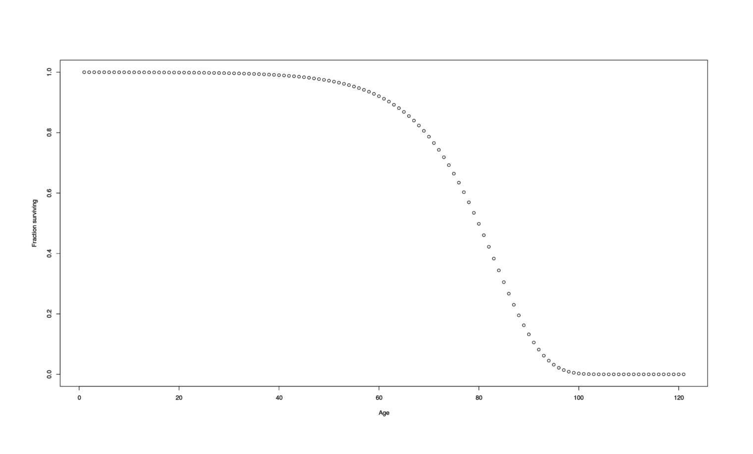
Population survival curve
It is also useful to draw random samples from a Gompertz-distribution of age-at-deaths, which can be used for generative model-related things like power simulations:
rgompertz <- function(n, RR=1) {
    ageHazards <- sapply(0:120, function(t) { H(t, RR) })
    ## for each possible age, randomly sample a life event according to that age's hazard;
    ## then the subject dies at the age at which their first FALSE is found.
    ## So `TRUE,TRUE,TRUE,FALSE,TRUE,FALSE` → died 4yo.
    deathAges <- replicate(n,
                  Position(`!`, sapply(ageHazards, function(h){sample(c(TRUE,FALSE), 1, prob=c(1-h, h))})))
    return(deathAges) }
## example uses:
mean(rgompertz(1000))
# [1] 77.705
mean(rgompertz(1000, RR=0.50))
# [1] 84.219
Converting Risk Reduction to Average Life Expectancy Gain
However, interpreting an RR/OR/STR isn’t as simple as “probability of death is reduced in each time period by 15%, we have average life expectancies of ~80, therefore, X will make me live an extra years”. (The intuition here is that death rates increase so much with time that a one-off reduction in each period doesn’t make a huge long-term difference. You can see that any constant intervention moves the curve up a little bit but does not flatten it.)
The Gompertz curve hazard can be multiplied by the RR to give a particular trajectory with that change in risk, and the mean can be obtained by integrating over a lifetime (more efficient than estimating by simulation using our rgompertz). Doing two such integrations, one with a baseline RR of 1 and one with the new RR, then gives the two different life expectancies, and subtraction indicates the net gain/loss:
lifeExpectancy <- function(RR, age1, age2) { integrate(function(t){S(t, RR) / S(age1, RR)},
                                                       age1, age2)$value }
lifeExpectancyGain <- function(RR, startingAge=0, endingAge=Inf)
                        { lifeExpectancy(RR, startingAge, endingAge) -
                           lifeExpectancy(1, startingAge, endingAge) }

## visualize:
rrs <- sort(c(seq(0.01,2,by=0.05), seq(0.95, 1.05, by=0.01)))
gainsVsRR <- data.frame(RR=rrs, Gain=sapply(rrs, lifeExpectancyGain))
plot(gainsVsRR, ylab="Gain (in years)")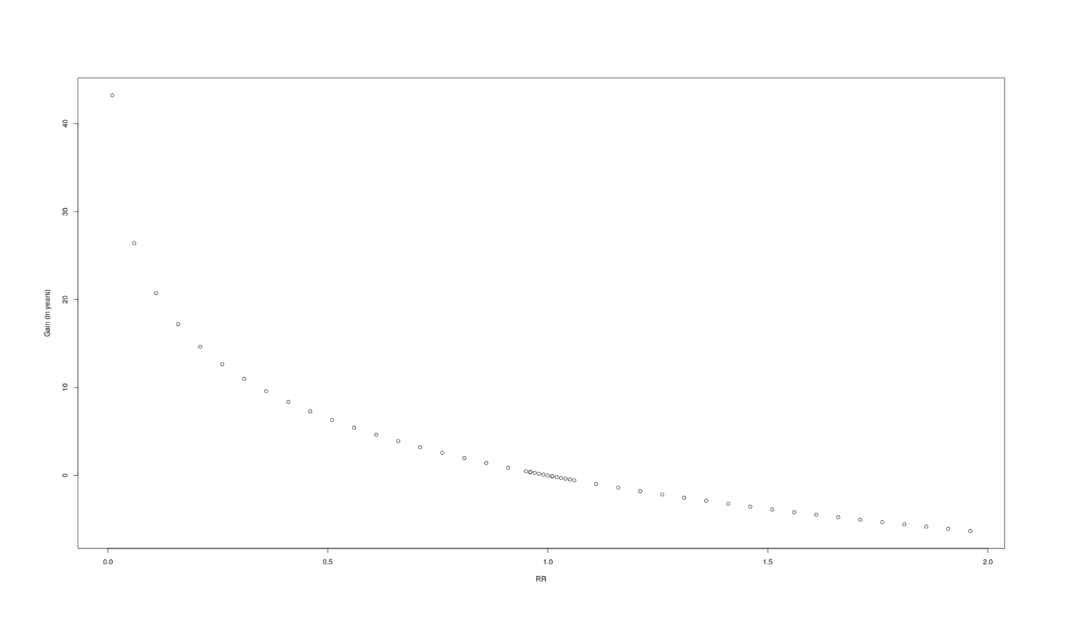
A graph of how many additional years a given change in RR causes.
RR |
Gain |
|---|---|
0.01 |
43.22 |
0.06 |
26.40 |
0.11 |
20.71 |
0.16 |
17.19 |
0.21 |
14.64 |
0.26 |
12.64 |
0.31 |
10.99 |
0.36 |
9.58 |
0.41 |
8.36 |
0.46 |
7.28 |
0.51 |
6.32 |
0.56 |
5.44 |
0.61 |
4.64 |
0.66 |
3.90 |
0.71 |
3.21 |
0.76 |
2.57 |
0.81 |
1.98 |
0.86 |
1.41 |
0.91 |
0.88 |
0.96 |
0.38 |
0.95 |
0.48 |
0.96 |
0.38 |
0.97 |
0.29 |
0.98 |
0.19 |
0.99 |
0.09 |
1.00 |
|
1.01 |
-0.09 |
1.01 |
-0.09 |
1.02 |
-0.19 |
1.03 |
-0.28 |
1.04 |
-0.37 |
1.05 |
-0.46 |
1.06 |
-0.55 |
1.11 |
-0.98 |
1.16 |
-1.39 |
1.21 |
-1.79 |
1.26 |
-2.17 |
1.31 |
-2.53 |
1.36 |
-2.88 |
1.41 |
-3.22 |
1.46 |
-3.55 |
1.51 |
-3.86 |
1.56 |
-4.17 |
1.61 |
-4.46 |
1.66 |
-4.75 |
1.71 |
-5.03 |
1.76 |
-5.30 |
1.81 |
-5.56 |
1.86 |
-5.82 |
1.91 |
-6.06 |
1.96 |
-6.31 |
If we plot a lot of samples of RR vs gain to get some intuition, it looks like a logarithmic curve, and indeed a linear model turns out to fit extremely well (r2= 0.9999), certainly good enough for our purposes, so if we needed better performance we could replace two integrals by 4 arithmetic operations:
summary(lm(Gain ~ log(RR), data=gainsVsRR))
#         Min          1Q      Median          3Q         Max
# -0.00110357 -0.00095014 -0.00049523  0.00025105  0.39525452
#
# Coefficients:
#                  Estimate    Std. Error      t value   Pr(>|t|)
# (Intercept)  0.0009609580  0.0002853556      3.36758 0.00077752
# log(RR)     -9.3742723770  0.0006917444 -13551.64204 < 2.22e-16
#
# Residual standard error: 0.01024382 on 1499 degrees of freedom
# Multiple R-squared:  0.9999918,   Adjusted R-squared:  0.9999918
# F-statistic: 1.83647e+08 on 1 and 1499 DF,  p-value: < 2.2204e-16
lifeExpectancyGainLogApproximation <- function(RR) { 0.0009609580 + -9.3742723770*log(RR) }
lifeExpectancyGain(0.85)
# [1] 1.523915331
lifeExpectancyGainLogApproximation(0.85)
# [1] 1.52445767
Anyway, with this conversion of risk to years of gained life, we can see how much bang we get:
lifeExpectancyGain(0.90)
# [1] 0.9879195324
lifeExpectancyGain(0.85)
# 1.523913984
lifeExpectancyGain(0.85) - lifeExpectancyGain(0.85, startingAge=30)
# [1] 0.02529745239
(0.02529745239 /  1.523913984 ) * 100
# [1] 1.660031515
lifeExpectancyGain(0.85) - lifeExpectancyGain(0.85, startingAge=60)
# [1] 0.2763949673
The back-loading of mortality means that a constant reduction in mortality risk like an RR of 0.85 would not deliver the naive expectation of 12 years but far less: ~1.6 years. On the plus side, this also means that if we wait to use an intervention until what might seem like ‘late’ in life (like age 30), we have not suffered a large opportunity cost (of ~40%) like one might think, but much less (~1.7%). The gains are minimal early on, and the opportunity cost only begins to really mount starting in one’s 50s or 60s, which has the important implication that such interventions will benefit younger people much less (at least when it comes to interventions which offer only a constant reduction in risk and do not affect the acceleration of mortality caused by the aging process itself) and so the risks are more likely to make interventions profitable.
Maximum Possible Profit
More generally, it would be interesting to get an idea of what is the most profit possible for any particular reduction in ACM, by granting the most favorable possible assumptions: certainty that the RR is exact, that the intervention is side-effect-less and free both to start and continue, and it can begin at birth if need be. For the plausible range of RRs, 0.5-1.0:
profitByAge <- function(t, RR=0.85, yearValue=50000, annualCost, startCost, probabilityPenalty=(1/3)) {
                (lifeExpectancyGain(RR, startingAge=t) * yearValue * probabilityPenalty) -
                                        (annualCost*lifeExpectancy(RR,t,Inf) + startCost) }

rrs <- seq(0.5,1,by=0.025)
startAge <- 0
data.frame(RR=rrs,
           Years=sapply(rrs, function(r) { lifeExpectancyGain(r, startAge) }),
           Maximum.Profit=sapply(rrs, function(r){profitByAge(startAge, RR=r, annualCost=0, startCost=0,
                                                              probabilityPenalty=1)}))
#       RR        Years Maximum.Profit
# 1  0.500 6.5010477923   325052.38962
# 2  0.525 6.0433308206   302166.54103
# 3  0.550 5.6069241021   280346.20511
# 4  0.575 5.1899323362   259496.61681
# 5  0.600 4.7907023355   239535.11678
# 6  0.625 4.4077834664   220389.17332
# 7  0.650 4.0398958538   201994.79269
# 8  0.675 3.6859046025   184295.23012
# 9  0.700 3.3447986050   167239.93025
# 10 0.725 3.0156733541   150783.66770
# 11 0.750 2.6977164037   134885.82019
# 12 0.775 2.3901950076   119509.75038
# 13 0.800 2.0924464396   104622.32198
# 14 0.825 1.8038691126    90193.45563
# 15 0.850 1.5239153307    76195.76654
# 16 0.875 1.2520850389    62604.25194
# 17 0.900 0.9879204526    49396.02263
# 18 0.925 0.7310014242    36550.07121
# 19 0.950 0.4809414268    24047.07134
# 20 0.975 0.2373840605    11869.20302
# 21 1.000 0.0000000000        0.00000
This provides upper bounds, and can help gauge plausibility of interventions for various variables - for example, if we were a 90-yo man considering embarking on caloric restriction, we might note that the upper bounds look like
# ...
# 13 0.800 2.0924464396   104622.32198
# 14 0.825 1.8038691126    90193.45563
# 15 0.850 1.5239153307    76195.76654
# 16 0.875 1.2520850389    62604.25194
# 17 0.900 0.9879204526    49396.02263
# 18 0.925 0.7310014242    36550.07121
# 19 0.950 0.4809414268    24047.07134
# 20 0.975 0.2373840605    11869.20302
# 21 1.000 0.0000000000        0.00000
Then we have to take into account the uncertainty that caloric restriction works at all in the extremely elderly (a halving is probably optimistic), the high probability its reduction in mortality will be relatively modest and in the 0.90s, the large financial & time costs of safely doing such a stringent diet (easily thousands of dollars in time and higher-quality food ingredients), the need to learn new recipes and count calories, the possible side-effects like increasing frailty & muscle loss… Given that the upper bound for plausible effect sizes is merely 1 year/$50k, it strikes me as extremely unlikely that such a man could justify CR.
We could also go the other direction and ask what is the worst RR that justifies a particular dollar cost using uniroot to find the zero of profitsByAge:
costToRR <- function (startingAge=30, annualCost, startCost=0, probabilityPenalty=1) {
  uniroot(f=function(r) {
          profitByAge(startingAge, RR=r, annualCost=annualCost, startCost=startCost,
                      probabilityPenalty=probabilityPenalty) },
          lower=.Machine$double.eps, upper=1)$root }
costToRR(annualCost=1000)
# [1] 0.9008035856
costToRR(annualCost=10)
# [1] 0.9989756733
Power Analysis
How many subjects does it take to detect a specified RR? This is useful for planning clinical trials but also in interpreting them. We can do simulation power analyses of an odds-ratio text on all-cause mortality by using rgompertz to generate a number of subjects’ death dates for different RRs (eg. 0.85 vs 1.0), counting how many deaths in each group fall within a specified followup period of years, and running some sort of analysis based on that data. (A more efficient design would be to simulate out a full survival curve and do a log-rank test on a Gompertz or nonparametric curve, but this requires individual-level data while most papers report only the OR; compare the Gompertz curve power analysis of Petrascheck & Miller 2017.)
gompertzSimulation <- function(RR, n1, n2, startingAge, followupYears) {
    experimental <- Filter(function(deathDate){deathDate>=startingAge}, rgompertz(n1, RR))
    control      <- Filter(function(deathDate){deathDate>=startingAge}, rgompertz(n2, 1))

    experimentalDeaths <- Filter(function(deathDate){deathDate<=(startingAge+followupYears)}, experimental)
         controlDeaths <- Filter(function(deathDate){deathDate<=(startingAge+followupYears)}, control)

    df <- data.frame(RR=RR,Start=startingAge, Followup=followupYears,
                     N1=length(experimental), N2=length(control),
                     N1.deaths=length(experimentalDeaths), N2.deaths=length(controlDeaths))
    return(cbind(df, data.frame(RR.observed=(df$N1.deaths/df$N1) /(df$N2.deaths/df$N2)))) }

gompertzPower <- function(RR, n1, n2, startingAge, followupYears, iters=100) {
    library(parallel)
    library(plyr)
    ldply(mclapply(1:iters, function(i) { gompertzSimulation(RR, n1, n2, startingAge, followupYears); }))
 }
Given a function to estimate power for a particular set of trial characteristics, we can also search for the sample size which would make a trial (or fixed-effect meta-analysis) of particular RR effects well-powered as a heuristic for what sort of sample sizes we should expect (remembering that being well-powered is neither necessary nor optimal for decision-making):
gompertzPowerSearch <- function (RR, startingAge=50, followupYears=10, targetPower=0.8, startingN=4000, iters=100, increment=200)  {
  n <- startingN
  nPower <- 0
  while (nPower < targetPower)  {
    n <- n+increment
    sims <- gompertzPower(RR, n, n, startingAge, followupYears, iters)
    pvalues <- sapply(1:nrow(sims),
              function(i) { prop.test(c(sims[i,]$N1.deaths, sims[i,]$N2.deaths), c(sims[i,]$N1, sims[i,]$N2),
                                      alternative="less")$p.value })
    nPower <- sum(pvalues<=0.05) / length(pvalues)
    }
  return(n)
}
startingN <- 4500
for (RR in seq(0.80, 0.95, by=0.01)) {
  n <- gompertzPowerSearch(RR, startingN=startingN)
  startingN <- n
  print(paste0("RR ", RR, "; necessary sample: ", n))
  }
RR |
Well-powered: 1 arm |
Total n |
|---|---|---|
0.80 |
4700 |
9400 |
0.81 |
6100 |
12200 |
0.82 |
6300 |
12600 |
0.83 |
6900 |
13800 |
0.84 |
7100 |
14200 |
0.85 |
8900 |
17800 |
0.86 |
9300 |
18600 |
0.87 |
11100 |
22200 |
0.88 |
12500 |
25000 |
0.89 |
15700 |
31400 |
0.90 |
18700 |
37400 |
0.91 |
21500 |
43000 |
0.92 |
28500 |
57000 |
0.93 |
34100 |
68200 |
0.94 |
46500 |
93000 |
0.95 |
68700 |
137400 |
Prior on RRs
Useful interventions are rare and our analyses should incorporate a skeptical informative prior reflecting our knowledge that it is highly unlikely that any particular intervention will genuinely increase life expectancy; in particular, RRs <0.5 (or >2.0) are rare. Since there are no previous compilations of randomized effects for interventions on all-cause mortality in healthy people to use for priors, I fall back on general-purpose but still informative skeptical priors found to work well across many problems by Gelman et al 2008 & Pedroza et al 2015: the Cauchy(0, 2.52) and Normal(0, 0.352) priors.
Vitamin D
A review of vitamin D meta-analyses reporting on all-cause mortality yields a meta-analytic result of RR=0.96 with little heterogeneity or signs of bias. Reproducing it as a Bayesian random-effects meta-analysis gives a posterior predictive probability P=84% that RR<1.0. The expected life expectancy gain is 0.33 years or $16,800, while total cost of vitamin D supplementation is estimated at $761, for a profit of $15,300. The probability of being profitable is estimated at P=83%. The optimal beginning age is 24yo.
Background
Vitamin D3 and vitamin D2 have been researched intensively ever since their discovery for possible benefits for a range of problems, starting with rickets and expanding from there to everything under the sun. Interest in vitamin D is sparked by many correlational results showing low levels of vitamin D in modern Western populations (unsurprising, given how little time people spend in the sun compared to historically) and how low levels correlate and predict with all sorts of bad things - particularly all-cause mortality.
The downside is that the literature is so large and heterogeneous that it’s hard to deal with and for many of the uses investigated, there is conflicting evidence. We are fortunate, however: the large research area of bone fractures/falls/osteoporosis in the elderly (collectively, leading causes of death & disability) means many (relatively) large RCTs in (relatively) healthy people are available with meaningful death rates reported. For particularly comprehensive reviews, see Newberry et al 2014 and Theodoratou et al 2014.
In addition, vitamin D3 also has considerable plausibility for being profitable: it can be taken in extremely large doses (>10-100x normal daily doses) without much sign of toxicity (leading to a fair number of trials which ensure compliance by just injecting mega-doses of vitamin D every month or year), hypervitaminosis D is rare and not usually fatal, side-effects are rare and minimal, it is already taken by many millions of healthy and sick people without noticeable problems, and vitamin D costs ~$15/year.
Causality
Quasi-Experimental
The 3 Mendelian Randomization studies I found show clear negatives to genetically lower vitamin D levels:
Levin et al 201214ya, “Genetic variants and associations of 25-hydroxyvitamin D concentrations with major clinical outcomes”
Examination of 141 single-nucleotide polymorphisms in a discovery cohort of 1514512ya white participants…Composite outcome of incident hip fracture, myocardial infarction, cancer, and mortality over long-term follow-up….Among Cardiovascular Health Study participants, low 25-hydroxyvitamin D concentration was associated with hazard ratios for risk of the composite outcome of 1.40 (95% CI, 1.12-1.74) for those who had 1 minor allele at rs7968585 and 1.82 (95% CI, 1.31-2.54) for those with 2 minor alleles at rs7968585. In contrast, there was no evidence of an association (estimated hazard ratio, 0.93 [95% CI, 0.70-1.24]) among participants who had 0 minor alleles at this single-nucleotide polymorphism.
Table 2 gives associations with all-cause mortality: 1.3 (1.0-1.6); 0.8 (0.7-1.0); 1.2 (0.9-1.5); 0.8 (0.6-1.1); 0.8 (0.6-1.0).
Trummer et al 201313ya, “Vitamin D and mortality: a Mendelian Randomization study”
a prospective cohort study of 3,316 male and female participants [total]…RESULTS: In a linear regression model adjusting for month of blood sampling, age, and sex, vitamin D concentrations were predicted by GC genotype (p < 0.001), CYP2R1 genotype (P = 0.068), and DHCR7 genotype (p < 0.001), with a coefficient of determination (r2) of 0.175. During a median follow-up time of 9.9 years, 955 persons (30.0%) died, including 619 deaths from cardiovascular causes. In a multivariate Cox regression adjusted for classical risk factors, GC, CYP2R1, and DHCR7 genotypes were not associated with all-cause mortality
Table 3: 0.95 (0.86-1.06), 1.00 (0.91-1.10); 0.94 (0.84-1.05);
Afzal et al 201412ya, “Genetically low vitamin D concentrations and increased mortality: Mendelian Randomization analysis in three large cohorts”:
95,766 white participants of Danish descent from three cohorts…The multi-variable adjusted hazard ratios for a 20 nmol/liter lower plasma 25-hydroxyvitamin D concentration were 1.19 (95% confidence interval 1.14 to 1.25) for all cause mortality…For DHCR7 and CYP2R1, we constructed an aggregate allele score of 0-4 as the sum of the number of 25-hydroxyvitamin D lowering alleles across the two genotypes in each gene….The hazard ratio per one DHCR7/CYP2R1 allele score increase was 1.02 (1.00 to 1.03; p = 0.03) for all cause mortality
RCTs
I searched Pubmed and Google Scholar on 2015-01-02 with the searches:
‘“vitamin D”[All Fields] AND ((“random allocation”[MeSH Terms] OR (“random”[All Fields] AND “allocation”[All Fields]) OR “random allocation”[All Fields] OR “randomized”[All Fields]) AND (“mortality”[Subheading] OR “mortality”[All Fields] OR “mortality”[MeSH Terms])) AND (Meta-Analysis[ptyp] AND “humans”[MeSH Terms])’
After reviewing hits and reading all the relevant looking papers and following citations, the most useful were:
Autier & Gandini 200719ya, “Vitamin D supplementation and total mortality: a meta-analysis of randomized controlled trials”:
We identified [k=]18 independent randomized controlled trials, including 57 311 participants. A total of 4777 deaths from any cause occurred during a trial size-adjusted mean of 5.7 years. Daily doses of vitamin D supplements varied 300–2000 IU. The trial size-adjusted mean daily vitamin D dose was 528 IU. In 9 trials, there was a 1.4- to 5.2-fold difference in serum 25-hydroxyvitamin D between the intervention and control groups. The summary relative risk for mortality from any cause was 0.93 (95% confidence interval, 0.87-0.99).
Barnard & Colon-Emeric 201016ya, “Extraskeletal effects of vitamin D in older adults: cardiovascular disease, mortality, mood, and cognition”:
Re-reports Autier & Gandini 200719ya and is redundant.
Elamin et al 201115ya, “Vitamin D and cardiovascular outcomes: a systematic review and meta-analysis”:
Vitamin D was associated with non-statistically-significant effects on the patient-important outcomes of death
[RR 0.96 (0.93-1.00); p = 0.08; k = 30]
Bolland et al 201115ya, “Calcium supplements with or without vitamin D and risk of cardiovascular events: reanalysis of the Women’s Health Initiative limited access dataset and meta-analysis”:
Patient-level data were available for 24 869 people in [k=]6 trials (WHI CaD and five randomized, placebo controlled trials of calcium supplements)…The hazard ratio for death (all causes) was 1.04 (0.95 to 1.14, p = 0.4).
Rejnmark et al 201214ya, “Vitamin D with calcium reduces mortality: patient level pooled analysis of 70,528 patients from eight major vitamin D trials”:
The IPD analysis yielded data on 70,528 randomized participants (86.8% females) with a median age of 70 (interquartile range, 62-77) yr. Vitamin D with or without calcium reduced mortality by 7% [hazard ratio, 0.93; 95% confidence interval (CI), 0.88-0.99]. However, vitamin D alone did not affect mortality, but risk of death was reduced if vitamin D was given with calcium (hazard ratio, 0.91; 95% CI, 0.84-0.98). The number needed to treat with vitamin D plus calcium for 3 yr to prevent one death was 151. Trial level meta-analysis (24 trials with 88,097 participants) showed similar results, i.e. mortality was reduced with vitamin D plus calcium (odds ratio, 0.94; 95% CI, 0.88-0.99), but not with vitamin D alone (odds ratio, 0.98; 95% CI, 0.91-1.06).
k = 8 & k = 24
Zheng et al 201313ya, “Meta-analysis of long-term vitamin D supplementation on overall mortality”:
Vitamin D therapy significantly decreased all-cause mortality with a duration of follow-up longer than 3 years with a RR (95% CI) of 0.94 (0.90-0.98). [k = 13] No benefit was seen in a shorter follow-up periods with a RR (95% CI) of 1.04 (0.97-1.12) [k = 29]
Zheng does not report the pooled RR of all studies. I calculate it at RR=0.981, p = 0.331
Lazzeroni et al 201313ya, “Vitamin D Supplementation and Cancer: Review of Randomized Controlled Trials”:
Focused on cancer, not all-cause mortality and so not relevant, but does note some methodological issues that apply to most vitamin D RCTs: subjects often do not take the provided supplements, and may be taking vitamin D on their own; the vitamin D doses used can vary widely; baseline levels of vitamin D in blood also can vary widely, which leads to both greater noise and, given the common U or J-shaped dose-response curves, might hide benefits or cause harm; vitamin D itself might interact with other drugs or supplements (eg. Lazzeroni et al note an apparent interaction with estrogen supplementation in the Women’s Health Initiative Trial).
Bjelakovic et al 201412ya (update of Bjelakovic et al 201115ya), “Vitamin D supplementation for prevention of cancer in adults”:
Vitamin D decreased all-cause mortality (1,854⁄24,846 (7.5%) versus 2,007⁄25,020 (8.0%); RR 0.93 (95% CI 0.88 to 0.98); p = 0.009; I2 = 0%; [k]=15 trials; 49,866 participants; moderate quality evidence), but TSA indicates that this finding could be due to random errors.
Bjelakovic et al 201412ya, “Vitamin D supplementation for prevention of mortality in adults”
Accordingly, 56 randomized trials with 95,286 participants provided usable data on mortality…Vitamin D decreased mortality in all 56 trials analysed together (5,920/47,472 (12.5%) vs 6,077/47,814 (12.7%); RR 0.97 (95% confidence interval (CI) 0.94 to 0.99); P = 0.02; I2 = 0%). More than 8% of participants dropped out. ‘Worst-best case’ and ‘best-worst case’ scenario analyses demonstrated that vitamin D could be associated with a dramatic increase or decrease in mortality. When different forms of vitamin D were assessed in separate analyses, only vitamin D3 decreased mortality (4,153/37,817 (11.0%) vs 4,340/38,110 (11.4%); RR 0.94 (95% CI 0.91 to 0.98); P = 0.002; I2 = 0%; 75,927 participants; 38 trials). Vitamin D2, alfacalcidol and calcitriol did not significantly affect mortality. A subgroup analysis of trials at high risk of bias suggested that vitamin D2 may even increase mortality, but this finding could be due to random errors. Trial sequential analysis supported our finding regarding vitamin D3, with the cumulative Z-score breaking the trial sequential monitoring boundary for benefit, corresponding to 150 people treated over five years to prevent one additional death. We did not observe any statistically-significant differences in the effect of vitamin D on mortality in subgroup analyses of trials at low risk of bias compared with trials at high risk of bias; of trials using placebo compared with trials using no intervention in the control group; of trials with no risk of industry bias compared with trials with risk of industry bias; of trials assessing primary prevention compared with trials assessing secondary prevention; of trials including participants with vitamin D level below 20 ng⧸mL at entry compared with trials including participants with vitamin D levels equal to or greater than 20 ng⧸mL at entry; of trials including ambulatory participants compared with trials including institutionalized participants; of trials using concomitant calcium supplementation compared with trials without calcium; of trials using a dose below 800 IU per day compared with trials using doses above 800 IU per day; and of trials including only women compared with trials including both sexes or only men.
Note that despite the almost identical author, date, & year, this differs from the other Bjelakovic et al 201412ya Cochrane review in focusing on mortality rather than cancer prevention.
Bolland et al 201412ya, “The effect of vitamin D supplementation on skeletal, vascular, or cancer outcomes: a trial sequential meta-analysis”:
k = 41, RR 0.96 (0.93-1.00)
Chowdhury et al 201412ya, “Vitamin D and risk of cause specific death: systematic review and meta-analysis of observational cohort and randomized intervention studies”:
In randomized controlled trials, relative risks for all cause mortality were 0.89 (0.80 to 0.99) for vitamin D3 supplementation and 1.04 (0.97 to 1.11) for vitamin D2 supplementation.
k = 22 total: k = 14 for vitamin D3 and k = 8 for vitamin D2.
Newberry et al 201412ya (update of Chung et al 200917ya), “Vitamin D and Calcium: A Systematic Review of Health Outcomes (Update)”:
For the re-analysis conducted in the original report, they excluded 5 of 18 trials in the Autier 200719ya meta-analysis: One trial was on patients with congestive heart failure,206 one was published only in abstract form,207 in one trial the controls also received supplementation with vitamin D, albeit with a smaller dose,208 and two trials used vitamin D injections.209,210 One additional eligible RCT (Lyons 200719ya)185 was identified and included in our meta-analysis….3 RCTs from the previous systematic review [based on Autier & Gandini 200719ya?] and an additional C rated RCT were included in our reanalysis. [k = 4] Three used daily doses that ranged between 400 and 880 IU, and one used 100,000 IU every 3 months. Our meta-analysis of the 4 RCTs (13,833 participants) shows absence of significant effects of vitamin D supplementation on all-cause mortality (RR = 0.97, 95% CI: 0.92, 1.02; random effects model). There is little evidence for between-study heterogeneity in these analyses.
As the selection is so limited, Newberry et al 201412ya is redundant with the others.
Theodoratou et al 201412ya, “Vitamin D and multiple health outcomes: umbrella review of systematic reviews and meta-analyses of observational studies and randomized trials”:
Vitamin D3: k = 9, 0.91 (0.82-1.02). Vitamin D2: k = 8, 1.04 (0.97-1.11). As well, an interesting comparison of randomized & correlational studies on the same outcomes:
10 (7%) outcomes were examined by both meta-analyses of observational studies and meta-analyses of randomized controlled trials: cardiovascular disease, hypertension, birth weight, birth length, head circumference at birth, small for gestational age birth, mortality in patients with chronic kidney disease, all cause mortality, fractures, and hip fractures (table 5⇓). The direction of the association/effect and level of statistical-significance was concordant only for birth weight, but this outcome could not be tested for hints of bias in the meta-analysis of observational studies (owing to lack of the individual data). The direction of the association/effect but not the level of statistical-significance was concordant in 6 outcomes (cardiovascular disease, hypertension, birth length, head circumference small for gestational age births, and all cause mortality), but only 2 of them (cardiovascular disease and hypertension) could be tested and were found to be free from hint of bias and of low heterogeneity in the meta-analyses of observational studies. For mortality in chronic kidney disease patients, fractures in older populations, and hip fractures [3], both the direction and the level of significance of the association/effect were not concordant.
Autier et al 201412ya, “Vitamin D status and ill health: a systematic review” (appendix):
Results of meta-analyses and pooled analyses consistently showed that supplementation could significantly reduce the risk of all-cause mortality, with relative risks ranging 0.93–0.96 (table 4)…Randomized controlled trials: The seven most recent meta-analyses summarised results of 88 randomized trials, some of which were included in several meta-analyses (table 4). We identified an additional 84 articles of randomized trials not included in published meta-analyses (table 5)…
Table 5 (studies not included in the listed meta-analyses) does not mention all-cause mortality, so only Autier et al is not reporting any new studies and is redundant with the others; Table 4 simply summarizes 3 past meta-analyses of ACM:
Elamin et al 201115ya: k = 30, RR=0.96 (0.93-1.00)
Bjelakovic et al 201115ya: k = 50 [error? should be k = 15?], RR=0.95 (0.91-0.99)
Rejnmark et al 201214ya: k = 62 [error? should be k = 8 & k = 24?] total, split between small and large (n > 1000) trials:
k = 38, RR=0.93 (0.88-0.99)
k = 24, RR=0.94 (0.88-0.99)
Avenell et al 201412ya (update of Avenell et al 200917ya, which is an update of Avenell et al 200422ya), “Vitamin D and vitamin D analogues for preventing fractures associated with involutional and post-menopausal osteoporosis”:
…mortality was not adversely affected by either vitamin D or vitamin D plus calcium supplementation ([k=]29 trials, 71,032 participants, RR 0.97, 95% CI 0.93 to 1.01)
“A Meta-Analysis of High Dose, Intermittent Vitamin D Supplementation among Older Adults”, Zheng et al 201511ya:
High dose, intermittent vitamin D therapy did not decrease all-cause mortality among older adults. The risk ratio (95% CI) was 1.04 (0.91-1.17)…Mortality data was available in seven trials [k = 7]
The overall thrust of the meta-analyses is that there is consistent and substantial evidence that regular vitamin D3 supplementation reduces all-cause mortality somewhere in the RR=0.90-1 range, that vitamin D2 may be worse but calcium seems irrelevant, and this effect seems to be general: the observable between-study heterogeneity is very small despite large differences in subject populations by gender, age, and dosage, and subgroup analyses do not find the effect confined to particular demographics or that a reduction in a particular disease is driving the ACM reduction (which while potentially due to lack of power, would be consistent with the generality of benefits in both the correlational and Mendelian Randomization studies).
The most comprehensive meta-analysis by my count is Bolland et al 201412ya, which pools k = 41 to get an estimate of RR 0.96 (0.93-1.00; p = 0.04) based on an experimental death rate of 3,824/40,379=0.0947 vs control death rate of 3,950/40,794=0.09682. The 41 studies are:
Inkovaara et al 198343ya, “Calcium, vitamin D and anabolic steroid in treatment of aged bones: double-blind placebo-controlled long-term clinical trial”
Corless et al 198541ya, “Do vitamin D supplements improve the physical capabilities of elderly hospital patients?”
Ooms et al 199531ya, “Prevention of bone loss by vitamin D supplementation in elderly women: a randomized double-blind trial”
Lips et al 199630ya, “Vitamin D supplementation and fracture incidence in elderly persons: A randomized, placebo-controlled clinical trial”
Komulainen et al 199828ya: “HRT and Vitamin D in prevention of non-vertebral fractures in postmenopausal women; a 5 year randomized trial” & “Prevention of femoral and lumbar bone loss with hormone replacement therapy and vitamin D3 in early postmenopausal women: a population-based 5-year randomized trial”
Meyer et al 200224ya, “Can vitamin D supplementation reduce the risk of fracture in the elderly? A randomized controlled trial”
Bischoff et al 200323ya, “Effects of vitamin D and calcium supplementation on falls: a randomized controlled trial”
Cooper et al 200323ya, “Vitamin D supplementation and bone mineral density in early postmenopausal women”
Latham et al 200323ya, “A randomized, controlled trial of quadriceps resistance exercise and vitamin D in frail older people: the Frailty Interventions Trial in Elderly Subjects (FITNESS)”
Trivedi et al 200323ya, “Effect of four monthly oral vitamin D3 (cholecalciferol) supplementation on fractures and mortality in men and women living in the community: randomized double blind controlled trial”
Avenell et al 200422ya, “The effects of an open design on trial participant recruitment, compliance and retention-a randomized controlled trial comparison with a blinded, placebo-controlled design”
Harwood et al 200422ya, “A randomized, controlled comparison of different calcium and vitamin D supplementation regimens in elderly women after hip fracture: the Nottingham Neck of Femur (NONOF) Study”
Aloia et al 200521ya, “A randomized controlled trial of vitamin D3 supplementation in African American women”
Flicker et al 200521ya, “Should older people in residential care receive vitamin D to prevent falls? Results of a randomized trial”
Grant et al 200521ya, “Oral vitamin D3 calcium for secondary prevention of low-trauma fractures in elderly people (Randomized Evaluation of Calcium Or vitamin D, RECORD): a randomized placebo-controlled trial”
Broe et al 200719ya, “A higher dose of vitamin D reduces the risk of falls in nursing home residents: a randomized, multiple-dose study”
Burleigh et al 200719ya, “Does vitamin D stop inpatients falling? A randomized controlled trial”
Lappe et al 200719ya, “Vitamin D and calcium supplementation reduces cancer risk: results of a randomized trial”
Lyons et al 200719ya, “Preventing fractures among older people living in institutional care: a pragmatic randomized double blind placebo controlled trial of vitamin D supplementation”
Smith et al 200719ya, “Effect of annual intramuscular vitamin D on fracture risk in elderly men and women—a population-based, randomized, double-blind, placebo-controlled trial”
Björkman et al 200818ya, “Vitamin D supplementation has minor effects on parathyroid hormone and bone turnover markers in vitamin D-deficient bedridden older patients”
Chel et al 200818ya, “Efficacy of different doses and time intervals of oral vitamin D supplementation with or without calcium in elderly nursing home residents”
Prince et al 200818ya, “Effects of ergocalciferol added to calcium on the risk of falls in elderly high-risk women”
Lips et al 201016ya, “Once-weekly dose of 8400 IU vitamin D(3) compared with placebo: effects on neuromuscular function and tolerability in older adults with vitamin D insufficiency”
Sanders et al 201016ya, “Annual high-dose oral vitamin D and falls and fractures in older women: a randomized controlled trial”
Glendenning et al 201214ya, “Effects of three-monthly oral 150,000 IU cholecalciferol supplementation on falls, mobility, and muscle strength in older postmenopausal women: a randomized controlled trial”
Chapuy et al 199234ya: “Vitamin D3 and calcium to prevent hip fractures in the elderly women” & “Effect of calcium and cholecalciferol treatment for three years on hip fractures in elderly women”
Dawson-Hughes et al 199729ya, “Effect of calcium and vitamin D supplementation on bone density in men and women 65 years of age or older”
Baeksgaard et al 199828ya, “Calcium and vitamin D supplementation increases spinal BMD in healthy, postmenopausal women”
Krieg et al 199927ya, “Effect of supplementation with vitamin D3 and calcium on quantitative ultrasound of bone in elderly institutionalized women: a longitudinal study”
Chapuy et al 200224ya, “Combined calcium and vitamin D3 supplementation in elderly women: confirmation of reversal of secondary hyperparathyroidism and hip fracture risk: the Decalyos II study”
Meier et al 200422ya, “Supplementation with oral vitamin D3 and calcium during winter prevents seasonal bone loss: a randomized controlled open-label prospective trial”
Porthouse et al 200521ya, “Randomized controlled trial of calcium and supplementation with cholecalciferol (vitamin D3) for prevention of fractures in primary care”
WHI trials 2006-07 47-49, “Calcium plus vitamin D supplementation and the risk of fractures” & “Calcium plus vitamin D supplementation and the risk of colorectal cancer” & “Calcium/vitamin D supplementation and cardiovascular events”
Bolton-Smith et al 200719ya, “Two-year randomized controlled trial of vitamin K1 (phylloquinone) and vitamin D3 plus calcium on the bone health of older women”
Salovaara et al 201016ya, “Effect of vitamin D(3) and calcium on fracture risk in 65- to 71-year-old women: a population-based 3-year randomized, controlled trial - the OSTPRE-FPS”
The meta-analysis itself can be reproduced given Bolland’s forest plot & table, Figure 5.
vitaminD <- read.csv(stdin(), header=TRUE,
                     colClasses=c("factor","integer","integer","integer","integer","integer","logical"))
Study, Year,E.deaths, E.n, C.deaths, C.n,Calcium
Inkovaara, 1983, 41, 181, 26, 146, FALSE
Corless, 1985, 8, 41, 8, 41, FALSE
Ooms, 1995, 11, 177, 21, 171, FALSE
Lips A, 1996, 223, 1291, 251, 1287, FALSE
Komulainen, 1998, 2, 232, 2, 232, FALSE
Meyer, 2002, 169, 569, 163, 575, FALSE
Bischoff, 2003, 1, 62, 4, 60, FALSE
Cooper, 2003, 0, 93, 1, 94, FALSE
Latham, 2003, 11, 121, 3, 122, FALSE
Trivedi, 2003, 224, 1345, 247, 1341, FALSE
Avenell, 2004, 4, 70, 3, 64, FALSE
Harwood, 2004, 24, 113, 5, 37, FALSE
Aloia, 2005, 1, 104, 2, 104, FALSE
Flicker, 2005, 76, 313, 85, 312, FALSE
Grant, 2005, 438, 2649, 460, 2643, FALSE
Broe, 2007, 5, 99, 2, 25, FALSE
Burleigh, 2007, 16, 101, 13, 104, FALSE
Lappe, 2007, 4, 446, 18, 734, FALSE
Lyons, 2007, 947, 1725, 953, 1715, FALSE
Smith, 2007, 355, 4727, 354, 4713, FALSE
Björkman, 2008, 27, 150, 9, 68, FALSE
Chel, 2008, 25, 166, 33, 172, FALSE
Prince, 2008, 0, 151, 1, 151, FALSE
Zhu, 2008, 0, 39, 2, 81, FALSE
Lips B, 2010, 1, 114, 0, 112, FALSE
Sanders, 2010, 40, 1131, 47, 1125, FALSE
Glendenning, 2012, 2, 353, 0, 333, FALSE
Inkovaara, 1983, 2, 353, 0, 333, TRUE
Chapuy A, 1992, 258, 1634, 274, 1636, TRUE
Dawson-Hughes, 1997, 2, 187, 2, 202, TRUE
Baeksgaard, 1998, 0, 80, 1, 80, TRUE
Krieg, 1999, 21, 124, 26, 124, TRUE
Chapuy B, 2002, 70, 389, 43, 194, TRUE
Harwood, 2004, 17, 75, 5, 37, TRUE
Meier, 2004, 0, 30, 1, 25, TRUE
Brazier, 2005, 3, 95, 1, 97, TRUE
Grant, 2005, 221, 1306, 217, 1332, TRUE
Porthouse, 2005, 57, 1321, 68, 1993, TRUE
WHI trials, 2006, 744, 18176, 807, 18106, TRUE
Bolton-Smith, 2007, 0, 62, 1, 61, TRUE
Zhu, 2008, 0, 39, 2, 41, TRUE
Salovaara, 2010, 15, 1718, 13, 1714, TRUE


library(metafor)
rem <- rma(measure="RR", ai=E.deaths, bi=(E.n-E.deaths), ci=C.deaths, di=(C.n-C.deaths),
           data=vitaminD, method="REML"); rem
# Random-Effects Model (k = 42; tau^2 estimator: REML)
#
# tau^2 (estimated amount of total heterogeneity): 0 (SE = 0.0015)
# tau (square root of estimated tau^2 value):      0
# I^2 (total heterogeneity / total variability):   0.00%
# H^2 (total variability / sampling variability):  1.00
#
# Test for Heterogeneity:
# Q(df = 41) = 36.5200, p-val = 0.6699
#
# Model Results:
#
# estimate       se     zval     pval    ci.lb    ci.ub
#  -0.0354   0.0186  -1.8990   0.0576  -0.0719   0.0011
## since I^2=0, this is equivalent to a fixed-effect meta-analysis:
fem <- rma(measure="RR", ai=E.deaths, bi=(E.n-E.deaths), ci=C.deaths, di=(C.n-C.deaths),
           data=vitaminD, method="FE"); fem
#
# Fixed-Effects Model (k = 42)
#
# Test for Heterogeneity:
# Q(df = 41) = 36.5200, p-val = 0.6699
#
# Model Results:
#
# estimate       se     zval     pval    ci.lb    ci.ub
#  -0.0354   0.0186  -1.8990   0.0576  -0.0719   0.0011
## 'metafor' works in log RR, so convert the log RR estimates back to RRs:
exp(-0.0719); exp(-0.0354); exp(0.0011)
# [1] 0.9306239536
# [1] 0.9652192513
# [1] 1.001100605
(Oddly, the per-study deaths/_n_s in the Bolland forest plot/table don’t add up to the claimed totals, but are short by a few dozen each; since the RR calculated by metafor works out to be about the same, I assume it has something to do with how Bolland decided to handle including multiple subgroups from studies and is not important.)
Turning from frequentist to Bayesian methods, we could take the fixed-effect at face-value and use a Bayesian proportion test, for example:
library(BayesianFirstAid)
bayes.prop.test(c(sum(vitaminD$E.deaths), sum(vitaminD$C.deaths)), c(sum(vitaminD$E.n), sum(vitaminD$C.n)))
#   Bayesian First Aid proportion test
#
# data: c(sum(vitaminD$E.deaths), sum(vitaminD$C.deaths)) out of c(sum(vitaminD$E.n), sum(vitaminD$C.n))
# number of successes:   4065,  4174
# number of trials:     42152, 42537
# Estimated relative frequency of success [95% credible interval]:
#   Group 1: 0.096 [0.094, 0.099]
#   Group 2: 0.098 [0.095, 0.10]
# Estimated group difference (Group 1 - Group 2):
#   0 [-0.0056, 0.0024]
# The relative frequency of success is larger for Group 1 by a probability
# of 0.203 and larger for Group 2 by a probability of 0.797.
Using BFA has the downside that an I2=0 doesn’t guarantee that there is no heterogeneity (it’d be surprising if there wasn’t) and gives an overly narrow predictive distribution, and BFA doesn’t easily include our informative priors. We can switch to bayesmeta which is easier to use than JAGS since it’s built on metafor:
library(bayesmeta)
brem <- bayesmeta(escalc(measure="RR", ai=E.deaths, bi=(E.n-E.deaths),
                                       ci=C.deaths, di=(C.n-C.deaths), data=vitaminD),
                  mu.prior.mean=0, mu.prior.sd=0.35^2)
brem
# ...ML and MAP estimates:
#                          tau             mu
# ML joint     3.878278037e-06 -0.03540646003
# ML marginal  0.000000000e+00             NA
# MAP joint    3.931136439e-07 -0.03460123602
# MAP marginal 0.000000000e+00 -0.03590402065
#
# marginal posterior summary:
#                     tau              mu
# mode      0.00000000000 -0.035904020655
# median    0.02518404476 -0.036069671647
# mean      0.03104981837 -0.036152849917
# sd        0.02543031565  0.022522077099
# 95% lower 0.00000000000 -0.080152143106
# 95% upper 0.08001681423  0.008768546338
## converting from log RRs to RR:
exp(c(-0.080152143106, -0.036152849917, 0.008768546338))
# [1] 0.9229759113 0.9644928596 1.0088071027

## posterior predictive distribution of RR values including heterogeneity
rrPP <- exp(brem$rposterior(10000, predict=TRUE)[,2])

## probability that vitamin D will reduce all-cause mortality in unobserved populations:
sum(rrPP<1) / length(rrPP)
# [1] 0.8489
Benefit
Expected life expectancy increase:
yearValue <- 50000
RR <- mean(rrPP)
years <- mean(sapply(rrPP, lifeExpectancyGain))
# [1] 0.336735595
years * yearValue
# 16836.77975
Hence, vitamin D supplementation could be worth <=$16.8k.
Cost
Financial
The meta-analyses do not have anything remotely near a consensus about dosage (nor do the correlational studies, despite much ink spilled), so it probably does not matter much. I have in the past purchased 360x5000IU vitamin D3 pills for $10.99, for an annual cost of $11.14. Taking a single pill takes perhaps a sixth of a minute, which again we value at $8/hr. So if we began taking at age 30:
moneyCost <- (10.99 / 360) * 365
timeCost <- ((1/10)/60) * 365.25 * 8
vitaminDAnnualCost <- moneyCost + timeCost
vitaminDTotalCost <- vitaminDAnnualCost * lifeExpectancy(RR, 30, Inf)
vitaminDTotalCost
# [1] 760.6887142
Dosage
To go into some more detail about the dosing issue, one of the more recent meta-analyses to discuss dose in connection with all-cause mortality, Autier et al 2014, says
…Results of meta-analyses and pooled analyses consistently showed that supplementation could significantly reduce the risk of all-cause mortality, with relative risks ranging 0.93–0.96 (table 4). Most trials included elderly women and a sizeable proportion of individuals were living in institutions. Decreases in risks of death were not associated with trial duration and baseline 25(OH)D concentration.13 Mortality reductions in trials that used doses of 10-20 μg [400-800IU] per day of vitamin D seemed greater than were reductions noted with higher doses.13,14
13. Bjelakovic G, Gluud LL, Nikolova D, et al. “Vitamin D supplementation for prevention of mortality in adults”. Cochrane Database Syst Rev 201115ya; 7: CD007470. [2014 update]
14. Rejnmark L, Avenell A, Masud T, et al. “Vitamin D with calcium reduces mortality: patient level pooled analysis of 70,528 patients from eight major vitamin D trials”. J Clin Endocrinol Metab 201214ya; 97: 2670-81.
(1μg=40IU, so 10μg=400IU, 20μg=800IU, and 125μg=5000IU.)
I’m not sure I agree. The mechanistic theory and correlations do not predict that 400IU is ideal, it doesn’t seem enough to get blood serum levels of 25(OH)D particularly higher, and I don’t read Rejnmark the same way: the Figure 3 forest plot, to me, shows that after correcting for Smith’s use of D2 rather than D3 (D2 usually performs worse), that there are too few studies using higher doses to make any kind of claim (Table 1; almost all the daily studies use <=20μg), and the studies which we do have tend to point to higher being better within this restricted range of dosages.
That said, I cannot prove that 5k IU is equally or more effective, so if anyone is feeling risk-averse or dubious on that score, they should stick with 800IU doses.
A year of daily 800IU doses costs almost the same as higher IU dosages since the vitamin D itself is only a small part of the cost of manufacturing. Alternately, if one is unconcerned about the different between daily and more intermittent doses (reasoning that due to the fat-solubility it should not make any difference), one could take a 5k IU dose on a weekly basis, thereby cutting the annual dose cost from ~$11 to ~$2.
Side-Effects
Due to rarity, effectively zero: the listed side-effects are all so rare or minor that I can’t come up with any reasonable estimate of cost.
Cost-Benefit
Bringing it all together for a 30yo considering vitamin D:
benefit <- lifeExpectancyGain(RR, startingAge=30) * yearValue
cost <- vitaminDTotalCost
benefit - cost
# [1] 15303.74835
Optimal Age
30 years turns out to be similar but later than the optimal age:
ages <- sapply(1:120, function(startingAge) {
         profitByAge(startingAge, RR=RR, vitaminDAnnualCost, 0, probabilityPenalty=1)})
optimalAge <- which.max(ages), optimalAge
# [1] 24
Sensitivity
What RR would wipe out the gains from vitamin D, and how likely is an RR that pessimistic?
zeroRR <- costToRR(startingAge=optimalAge, annualCost=vitaminDAnnualCost); zeroRR
# [1] 0.9981691406
sum(rrPP<zeroRR) / length(rrPP)
# [1] 0.8356
The window of unprofitability is so narrow that it doesn’t much change the probability.
Metformin
Metformin is a standard drug prescribed to diabetics since the 1950s, known for helping control blood sugar while being cheap and safe; it has been used by scores of millions of people. Alongside the blood sugar benefits, there appear to be other benefits relating to cancer and cardiovascular health, and possibly even all-cause mortality. There is enough public interest that I heard of it, and as it passes the sniff test, I decided to look into it further.
Overall, metformin is promising and under my set of assumptions, profitable for people aged >=45yo to use. This, however, entirely hinges on one’s evaluation of the credibility of the correlational evidence and ability to tolerate the surprisingly common & unpleasant side-effects like diarrhea.
Causality
Metformin has not been much tested in healthy adult populations, although there are a few anecdotes of prophylactic use (eg. James Watson) and a good deal of media attention has been given to a trial planned to launch in 2016: “Targeting Aging with Metformin” (TAME; profile of proponent Barzilai, interview, Nature article3, Barzilai et al 2016 advocacy paper). There are some meta-analyses of past clinical trials of diabetic patients, which include estimates for ACM. Interpretation is difficult due to generally small numbers of deaths, differences in what metformin was being compared to, and the generally diseased subjects, but the picture looks mixed:
Saenz et al 200521ya, “Metformin monotherapy for type 2 diabetes mellitus”; withdrawn by the Cochrane Collaboration (apparently due to obsolescence)
Selvin et al 200818ya, “Cardiovascular outcomes in trials of oral diabetes medications: a systematic review”
Metformin vs anything, RR=0.81.
Lamanna et al 201115ya, “Effect of metformin on cardiovascular events and mortality: a meta-analysis of randomized clinical trials”
RR=0.97 in active-comparator trials and 1.074 in placebo trials; overall, too underpowered to detect ACM of the plausible effect sizes but did find a trend towards larger reductions in longer trials.
Stevens et al 201214ya, “Cancer outcomes and all-cause mortality in adults allocated to metformin: systematic review and collaborative meta-analysis of randomized clinical trials”
ACM was split by comparison to placebo and comparison to another diabetic drug: 0.97 & 0.94.
Campbell et al 2017, “Metformin reduces all-cause mortality and diseases of aging independent of its effect on diabetes control: A systematic review and meta-analysis”:
Diabetics taking metformin had significantly lower all-cause mortality than non-diabetics (hazard ratio (HR)= 0.93, 95%CI 0.88-0.99), as did diabetics taking metformin compared to diabetics receiving non-metformin therapies (HR= 0.72, 95%CI 0.65-0.80), insulin (HR=0.68, 95%CI 0.63-0.75) or sulphonylurea (HR= 0.80, 95%CI 0.66-0.97).
Some of the biochemical & animal experimental background suggesting benefits may be generalizability to healthy people, with proposals that metformin is mimicking caloric restriction by subtly reducing efficiency of mitochondria, making the body think it is in a food-scarce state; however, if this is true, it may also be redundant with other interventions like intermittent fasting or fasting-mimicking drugs or exercise (there are 2 small studies suggesting, like antioxidants, metformin may interfere with exercise benefits, highlighted by the critical discussion Glossman & Lutz 2019). TAME seems to be prompted in part by Bannister et al 201412ya, “Can people with type 2 diabetes live longer than those without? A comparison of mortality in people initiated with metformin or sulphonylurea monotherapy and matched, non-diabetic controls”, a very large but nevertheless correlative result. There also appears to not be much consistency in the correlation results, with competing meta-analyses on various permutations of comparisons.
So I will apply my proposed correlation!=causality correction of 33% to deflate the expected value.
Benefit
We know metformin won’t increase lifespans by 40% like some mice or make one live to 120, and probably also offers only a constant reduction in risk without decreasing the acceleration of risk, if for no other reason than hundreds of millions of people have taken metformin over the past century yet no gerontologist has ever noticed a massive overrepresentation of diabetics among centenarians. The actual effect size estimates from the abstract of Bannister et al 201412ya (emphasis added):
We identified 78 241 subjects treated with metformin, 12 222 treated with sulphonylurea, and 90 463 matched subjects without diabetes. This resulted in a total, censored follow-up period of 503 384 years. There were 7498 deaths in total, representing unadjusted mortality rates of 14.4 and 15.2, and 50.9 and 28.7 deaths per 1,000 person-years for metformin monotherapy and their matched controls, and sulphonylurea monotherapy and their matched controls, respectively. With reference to observed survival in diabetic patients initiated with metformin monotherapy [survival time ratio (STR) = 1.0], adjusted median survival time was 15% lower (STR = 0.85, 95% CI 0.81-0.90) in matched individuals without diabetes and 38% lower (0.62, 0.58-0.66) in diabetic patients treated with sulphonylurea monotherapy.
STR isn’t quite an RR but it’s similar:
The log-logistic model resulted in the best fit in terms of AIC, and the adequacy of this distribution was further assessed by plotting appropriately transformed non-parametric estimates against time. The log-logistic survival model provides beta coefficients that equal the difference in log survival time between groups or for continuous predictors. Exponentiation of the beta coefficient gives the ratio between median survival times, known as the survival time ratio (STR), or acceleration factor. STRs less than 1 represent a decrease in survival time; values greater than 1 represent prolonged survival.
…In total, there were 7498 deaths, corresponding to an unadjusted event rate of 18.1 deaths per 1,000 person-years. Unadjusted event rates were highest in the sulphonylurea group and lowest in the metformin group (50.9 versus 14.4 per 1,000 person-years, respectively; p < 0.001; Table 2). Unadjusted event rates were higher in sulphonylurea-treated patients than in their matched, non-diabetic controls (50.9 versus 28.7 per 1,000 person-years, respectively; p < 0.001) but, surprisingly, were lower in those treated with metformin than in their matched controls (14.4 versus 15.2 per 1,000 person-years, respectively; p = 0.054). Unadjusted event rates were lowest in people aged <60 years at index date and highest for people aged >70 years for both diabetic and control subjects.
So I think if we wanted to convert to something else, STR has already done the denominator for us and we just divide 14.2 / 15.2 to get the raw RR of 0.93, which is not as good as the quoted STR of 0.85 (0.81-0.90), indicating that the covariates do differ a bit systematically? Looking at table 1, the metformin group seems to have been previously treated for many more disorders, explaining why the models think metformin is so good (because the metformin users should be dying off faster yet have a similar death rate as the healthy controls) Table 2 gives overall figures for all-cause mortality: n = 78241, 2663 deaths in metformin (); n = 78241, 2669 deaths in their controls (2,669/78,241=0.03411254969) (=0.9977519669). Pooling in the sulphonylurea controls as well: n = 748 deaths plus the 2669 other controls, total controls n = 90463, total deaths 3417 (3417/90,463=0.03777234892) (=0.9010788188). So that verifies the RR of 0.93 since the difference between 0.90 and 0.93 is probably due to the differences in total followup years.
An RR of 0.85/0.90 gets us around a year, which converting to dollars:
yearValue <- 50000
lifeExpectancyGain(0.90) * yearValue
# [1] 49396.02263
lifeExpectancyGain(0.85) * yearValue
# [1] 76195.76654
Or $50k-$76k.
Cost
Financial
Metformin is said to be very cheap. How cheap is cheap?
Bannister et al 201412ya doesn’t give dosages or look for a dose-response curve but since it’s drawing on clinical records, the diabetics must be using conventional dosages. Drugs.com gives a maintenance dose of 200026yamg/daily; the Mayo Clinic says not usually more than 2000–2500mg/daily; the anti-aging quacks tend to suggest ~1,000 mg/daily for non-diabetics; the MILES protocol calls for 1700326yamg/daily. I’ll use 200026yamg/daily here, which is 4x500mg doses.
GoodRx says that a number of large American chains, including Walmart & Target & Sam’s Club, will sell 60x500mg for $4. It’s unclear if this includes sales tax, so I will tack on an additional 5% for that. This is 15 days’ worth at 2000mg/daily, so a month’s supply is $8.4, and an annual supply is $102. For the time/effort of regular consumption, I’ll estimate it at half a minute a day and $8/hr. (Metformin has a shelf-life of 5 years so at least in theory one could buy large batches and then the shopping time is trivial.) If we start at age 30, then without any discounting, we can expect to pay for metformin for a number of years (increased, of course, by our metformin usage):
unitDoses <- (60*500) / 2000
unitCost <- 4 * 1.05
annualPurchases <- 365.25 / unitDoses
moneyCost <- unitCost * annualPurchases
timeCost <- (0.5/60) * 8 * 365.25
metforminAnnualCost <- moneyCost + timeCost; metforminAnnualCost
# [1] 126.62
Side-Effects
The direct monetary cost of metformin is so minimal that it’s almost certainly outweighed by the inconvenience of purchasing & regularly using it, and by any side-effects one might experience. Side-effects are a more serious concern: while considered safe and a net gain from the point of view of all-cause mortality, that just means the side-effects are relatively rare or nonfatal but metformin might still be unpleasant enough, or produce long-lasting reductions in quality of life which negate much of the gain. (It would not be much of an improvement to halve one’s risk if, in exchange, one becomes a quadriplegic.)
Drugs.com provides some percentage breakdowns after noting that many problems can be avoided by gradual increases in dosage or go away spontaneously
Metabolic:
Common (1% to 10%): Hypoglycemia
Very rare (less than 0.01%): Lactic acidosis[Ref]
Gastrointestinal:
Very common (10% or more): Diarrhea (53.2%), nausea/vomiting (25.5%), flatulence (12.1%)
Common (1% to 10%): Indigestion, abdominal discomfort, abnormal stools, dyspepsia, loss of appetite[Ref]
Hematologic: Very rare (less than 0.01%): Subnormal vitamin B12 levels[Ref]
Other: Common (1% to 10%): Asthenia, chills, flu syndrome, accidental injury[Ref]
Hepatic: Very rare (less than 0.01%): Liver function test abnormalities, hepatitis[Ref]
Cardiovascular: Common (1% to 10%): Chest discomfort, flushing, palpitation[Ref]
Dermatologic
Common (1% to 10%): Rash, nail disorder, increased sweating
Very rare (less than 0.01%): Erythema, pruritus, urticaria[Ref]
Endocrine: Frequency not reported: Reduction in thyrotropin (TSH) levels[Ref]
Immunologic: Very common (10% or more): Infection (20.5%)[Ref]
Musculoskeletal: Common (1% to 10%): Myalgia[Ref]
Nervous system: Common (1% to 10%): Lightheadedness, taste disturbances[Ref]
Psychiatric: Common (1% to 10%): Headache[Ref]
Respiratory: Common (1% to 10%): Rhinitis[Ref]
Most of these seem to be relatively minor or temporary, and the GI problems can be reduced by splitting up doses & taking with food; if they persist, a prophylactic user could simply discontinue metformin. (The FDA prescribing information notes in one trial, 6% of the metformin subjects had to stop because the diarrhea was so bad. Net attrition/dropout rates in metformin studies vary so much that they’re not helpful and not all of it will have to do with metformin reducing the daily quality of life through side-effects, but overall they look like 10-40% would be a reasonable guess.) Discontinuation would be too bad since then one doesn’t gain the benefits, but one won’t have lost too much besides perhaps a few weeks of severe diarrhea and a month or two of wasted metformin pills, so it’s not too bad. You might think we would have to incorporate a penalty of 10-40% to the expected value - if there’s a 10-40% chance the metformin is useless, shouldn’t we multiply the mortality benefit by 0.1-0.4? - but that’s only if we have no way of knowing the metformin is useless and we are considering the scenario in which we take it for the rest of our life even while it’s useless. In this case, because we know quickly if we can handle metformin or not, we only need to consider the upfront cost of the month of diarrhea. (So more formally: the expected value is lower, but the Value of Information is higher because once one starts metformin and the GI problems either turn out to not be so bad or to go away, the expected value then increases substantially now that one knows one can take metformin without problem.)
The main side-effect mentioned as potentially fatal is lactic acidosis—for example, of the 12 New Zealand cases 1977–21199828ya, 8 were fatal & the FDA prescribing information estimates 50%, which does not sound fun. On the other hand, lactic acidosis seems to be an acute disorder whose primary effect would be killing you, so it should already be taken care of by working with a reduction in all-cause mortality (that is, even if you are more likely to die by lactic acidosis, the metformin must be sparing you even more gruesome deaths and on average it’s still helpful). And the lactic acidosis rates (2-9 per 100,000 person-years, so at 50 years of usage as prophylactic, a risk of =0.003) may simply reflect the pre-existing morbidity of diabetics and not caused by metformin, and so not a concern at all.
So for side-effects, I think we can sum it up as a month or two of diarrhea, which is unpleasant but not that big a deal. I wouldn’t pay more than $50/day or so to get rid of some diarrhea, which over two months is $3,000, but that’s somewhat unlikely.
metforminStartCost <- 3000
metforminTotalCost <- metforminStartCost + metforminAnnualCost * lifeExpectancy(0.85, 30, Inf)
metforminTotalCost
# [1] 9164.222177
<$9.2k is a little under an order of magnitude smaller than the more conservative RR estimate, giving a gain of $69k for RR=0.85.
Cost-Benefit
Bringing it all together for a 30yo considering metformin:
benefit <- lifeExpectancyGain(0.85, startingAge=30) * yearValue * (1/3)
benefit - metforminTotalCost
# [1] 15812.74246
So metformin use is probably profitable for our 30yo.
Optimal Age
What about other ages? In fact, is there an optimal age at which to start, or should we be feeding little kids metformin too? Rewriting to generalize it, we can compute the profit for if we started at all ages:
ages <- sapply(1:120, function(startingAge) { profitByAge(t=startingAge, RR=0.85, yearValue=yearValue,
                                                          annualCost=metforminAnnualCost,
                                                          startCost=metforminStartCost,
                                                          probabilityPenalty=(1/3))})
ages
#   [1] 12581.36678184 12704.60247164 12827.51331458 12950.06734382 13072.23497395 13193.97822375
#   [7] 13315.25955302 13436.03553162 13556.25972902 13675.88249331 13794.84959193 13913.10174786
#  [13] 14030.57465454 14147.19877297 14262.56843491 14377.59313608 14491.19343288 14603.60417087
#  [19] 14714.72213847 14824.49779567 14932.62516230 15039.16033901 15143.90179637 15246.69929498
#  [25] 15347.39132485 15445.80840422 15541.75256433 15635.03632321 15725.44232215 15812.74246206
#  [31] 15896.69274016 15977.03622060 16053.49182110 16125.76969995 16193.55704406 16256.53548802
#  [37] 16314.32235685 16366.58143711 16412.91897286 16452.92599097 16486.17295649 16512.21623495
#  [43] 16530.59232830 16540.81861554 16542.39575833 16534.80739374 16517.52441118 16490.00437695
#  [49] 16451.69477821 16402.03608769 16340.46418394 16266.41385753 16179.32414828 16078.64173013
#  [55] 15963.82659990 15834.35747000 15689.73792729 15529.50334258 15353.22772268 15160.53106518
#  [61] 14951.08725079 14724.63218759 14480.97195447 14219.99094268 13941.65997415 13646.04417437
#  [67] 13333.31034505 13003.73373668 12657.70393148 12295.72850887 11918.44019624 11526.59453544
#  [73] 11121.07254740 10702.87925221 10273.14006106  9833.09512729  9384.09165549  8927.57401957
#  [79]  8465.07171100  7998.18524842  7528.57023589  7057.91974619  6587.94582834  6120.35841826
#  [85]  5656.84891652  5199.06318619  4748.58831275  4306.93008014  3875.49621238  3455.58095505
#  [91]  3048.34081949  2654.83557034  2275.91635712  1912.32384346  1564.63525304  1233.27268149
#  [97]   918.50921796   620.47329414   339.15724767    74.42696583  -173.96624441  -406.37341118
# [103]  -623.23364355  -825.06251102 -1012.43660004 -1185.98112738 -1346.35743240 -1494.25164331
# [109] -1630.36275346 -1755.39535284 -1870.04919810 -1975.01316139 -2070.95896128 -2158.53660863
# [115] -2238.37032302 -2311.05585076 -2377.15851698 -2437.21167794 -2491.71755097 -2541.14436644
max(ages)
# [1] 16542.39576
optimalAge <- which.max(ages); optimalAge
# [1] 45
Apparently there is an optimal age - and it’s not 30yo but 45yo (metformin is profitable enough that starting too early, rather than never, is still a good idea). So quite aside from waiting for better information like the MILES results, our hypothetical 30yo still should wait a long time before starting to use metformin. Also unsurprising is that ~90yo, mortality rates become so high that the metformin reduction yields such a small absolute gain of time that it can no longer offset the fixed absolute cost of metformin.
While $18k may not sound like that much on an individual level, it’s substantial (<$1.42t over all people currently 55+) on a societal scale:
## multiply maximal benefit by the total number of
## Americans >=55yo according to http://www.indexmundi.com/united_states/age_structure.html :
ages[which.max(ages)] * (19309019+20720284+20304644+25874360)
# [1] 1426091932050
The estimate is so small because we use a small estimate of the value of 1 QALY; Murphy & Topel 2005, using a much more sophisticated calculation and more realistic QALY estimates, note that “A 10% reduction in all-cause mortality [RR=0.90] would have a present discounted social value of $18.5 trillion.”
Sensitivity
We can also use the formula to ask how small (close to 1) the RR must be before, given the specified purchase & side-effect costs, there is no longer any age at which metformin is profitable:
costToRR(startingAge=optimalAge, annualCost=metforminAnnualCost, startCost=metforminStartCost,
         probabilityPenalty=(1/3))
# [1] 0.9520242072
So if one doesn’t believe the true causal ACM RR is <=0.95, then metformin use may not be advisable.
TAME Power Analysis
Using the previously defined gompertzPower function, we can ask a question like: assuming a clinical trial is investigating a claimed RR of 0.85, plans to enrol 3000 people aged 70yo, so presumably 1500 in each arm, and will followup for 5 years (a trial which bears a certain resemblance to plans for TAME); how often would the observed RR<1.0?
df0.85 <- gompertzPower(0.85, 1000, 1000, 50, 10, 100)
table(df0.85$RR.observed<1.0)
# FALSE  TRUE
#   22    78
Let’s consider something more plausible like the baby aspirin or some metformin estimates, an RR of 0.94:
df0.94 <- gompertzPower(0.94, 1500, 1500, 70, 5, 1000)
table(df0.94$RR.observed<1.0)
# FALSE  TRUE
#  236   764
76% power is likewise still acceptable. But just because a clinical trials plans to enrol n = 3000 doesn’t mean they will succeed, as there is always attrition, and attrition can be severe depending on how unpleasant the side-effects are; for metformin, for example, the attrition could easily be 30%:
df0.94attrit <- gompertzPower(0.94, 1500*0.70, 1500*0.70, 70, 5, 1000)
table(df0.94attrit$RR.observed<1.0)
# FALSE  TRUE
#   254   746
Knocking us back to 74%. So under more realistic assumptions about attrition and effect sizes, there’s a good chance that there would not be a correct signed result. Finally, we could consider the probability that we would get both a RR in the desired direction and the difference would be large enough to be statistically-significant at p < 0.05 when treated as a two-proportion problem:
df <- df0.94attrit
pvalues <- sapply(1:nrow(df),
            function(i) { prop.test(c(df[i,]$N1.deaths, df[i,]$N2.deaths), c(df[i,]$N1, df[i,]$N2),
                                    alternative="less")$p.value })
table(pvalues<=0.05)
# FALSE  TRUE
#  890   110
So it is highly unlikely (~10%) we could expect the realistic trial to deliver a statistically-significant reduction in mortality. (This lack of power for statistical-significance on ACM may be why the TAME investigators talk primarily about looking for reductions in cancer/heart attacks/strokes: as more common events than death, reductions will show up more clearly there, as they do in past metformin trials.) We don’t necessarily care about statistical-significance, since this is a decision-analysis approach: our question is whether the gained data shifts the posterior probability enough to change the optimal decision. But it’s good to have an idea of power in that sense to make it easier to interpret the research article & media reports (eg. the trial might be a ‘failure’ from the point of view of statistical-significance, even as it increases the profitability of using metformin).
If we really wanted 80% power for p < 0.05, how big a sample do we need? In this case, it turns out to be ~7500 per arm (after any attrition) or ~15k total.
Such large RCTs are difficult to run and motivate the search for quicker & more continuous measures, like Horvath’s epigenetic clock; unfortunately, biomarkers have a bad track record of measuring causal effects on the hard endpoints of interest, such as mortality. Epigenetic clocks don’t always work (eg. Thompson et al 2018) but there’s evidence suggesting they will (see José Luis’s discussion) and plausible interventions do seem to reduce epigenetic clocks (Fahy et al 2019, Fitzgerald et al 2020), so we’ll see.
See Also
External Links
“The economic value of targeting aging”, Scott et al 2021
A History of Life-Extensionism In The Twentieth Century, Stambler 2014
Global Burden of Disease: total DALYs lost by cause in the USA, 2016
“The quest to slow aging through drug discovery”, Partridge et al 2020
Pooled experimental arm death rate: =0.1143770118, control death rate =0.1164899196; then the test of difference:
prop.test(c((1175+3693), (1118+3880)), c((8809+33752), (9193+33712)))↩︎Or to put it more concretely, =86 excess deaths in the control group, who did not take vitamin D.↩︎
“Plans call for the trial to enrol 3,000 people aged 70-80 years at roughly 15 centres around the United States. The trial will take 5-7 years and cost US$50 million, Barzilai estimates, although it does not yet have funding.” There is also the Metformin in Longevity Study/MILES, but the pre-registration indicates it will be aimed at gene expression changes and too short-term for mortality differences.↩︎