LWer Effective Altruism donations, 2013–2014
Analysis of 2013–2014 LessWrong survey results on how much more self-identified EAers donate suggests low median donation rates due to current youth and low incomes.
A LW critic noted that the annual LW survey reported a median donation for “effective altruists” of $0, though the EA movement encourages strongly donations. I look closer at the 2013–2014 LW surveys and find in multiple regression that identifying as an EA does predict more donations after controlling for age and income, suggesting that the low EA median donation may be due to EAers having low income and youth (eg. being a student) rather than being unusually or even averagely selfish.
From “Portrait of EAs I know”, su3su2u1:
But I note from googling for surveys that the median charitable donation for an EA in the Less Wrong survey was 0.
Two years ago I got a paying residency, and since then I’ve been donating 10% of my salary, which works out to about $5,000 a year. In two years I’ll graduate residency, start making doctor money, and then I hope to be able to donate maybe eventually as much as $25,000 - $50,000 per year. But if you’d caught me five years ago, I would have been one of those people who wrote a lot about it and was very excited about it but put down $0 in donations on the survey.
If self-reported EAers donate a similar total/average amount as the non-EAers, this would imply that the respondents are likely hypocrites and that the movement is not succeeding in its goals. (While there are ways to contribute beyond donating money and there are legitimate reasons to donate only small amounts, it’s clear that for most people the optimal approach is donating money and in general First Worlders, particularly intelligent ones, can spare a large fraction of their income without dying or catastrophic loss of their quality of life.)
Data
The LW survey run by Yvain has, in the 201313ya and 201412ya surveys (but not previously), asked one or two questions about whether respondents self-identify as Effective Altruists and also how much they have donated that year to charity. The surveys also ask if one has responded to a previous survey, and ask about various things that might plausibly predict donations: employment status, profession, educational attainment, age, and of course, income.
So to investigate the claim of su3su2u1 that median self-reported donation is $0 and Yvain’s claims that donations increase substantially with age & EAers are in the low-income/age portion of their lives, we can
combine the 201313ya & 201412ya surveys for maximal data, filtering out people who answered both surveys
include year as a fixed effect in case of temporal changes
log-transform heavily-skewed monetary variables like donations & income
test the simplest possible form of su3su2u1’s claim using a non-parametric test of medians between EAers/non-EAers
and then try more sophisticated regressions, regressing the various demographic factors on log-donations, to see what the EA factor predicts after including the others as predictors (I also try treating the two EA questions as measures of a latent variable of EAness, which turns out to not much matter)
Analysis
Preparation
Data preparation:
set.seed(2015-05-13)
survey2013 <- read.csv("https://gwern.net/doc/lesswrong-survey/2013.csv", header=TRUE)
survey2013$EffectiveAltruism2 <- NA
s2013 <- subset(survey2013, select=c(Charity,Effective.Altruism,EffectiveAltruism2,Work.Status,
                                     Profession,Degree,Age,Income))
colnames(s2013) <- c("Charity","EffectiveAltruism","EffectiveAltruism2","WorkStatus","Profession",
                     "Degree","Age","Income")
s2013$Year <- 2013
survey2014 <- read.csv("https://gwern.net/doc/lesswrong-survey/2014.csv", header=TRUE)
s2014 <- subset(survey2014, PreviousSurveys!="Yes", select=c(Charity,EffectiveAltruism,EffectiveAltruism2,
                                                             WorkStatus,Profession,Degree,Age,Income))
s2014$Year <- 2014
survey <- rbind(s2013, s2014)

# replace empty fields with NAs:
survey[survey==""] <- NA; survey[survey==" "] <- NA

# convert money amounts from string to number:
survey$Charity <- as.numeric(as.character(survey$Charity))
survey$Income <- as.numeric(as.character(survey$Income))
# both Charity & Income are skewed, like most monetary amounts, so log transform as well:
survey$CharityLog <- log1p(survey$Charity)
survey$IncomeLog <- log1p(survey$Income)

# age:
survey$Age <- as.integer(as.character(survey$Age))
# prodigy or no, I disbelieve any LW readers are <10yo (bad data? malicious responses?):
survey$Age <- ifelse(survey$Age >= 10, survey$Age, NA)

# convert Yes/No to boolean TRUE/FALSE:
survey$EffectiveAltruism <- (survey$EffectiveAltruism  == "Yes")
survey$EffectiveAltruism2 <- (survey$EffectiveAltruism2  == "Yes")
summary(survey)
##     Charity           EffectiveAltruism EffectiveAltruism2                            WorkStatus
##  Min.   :     0.000   Mode :logical     Mode :logical      Student                         :905
##  1st Qu.:     0.000   FALSE:1202        FALSE:450          For-profit work                 :736
##  Median :    50.000   TRUE :564         TRUE :45           Self-employed                   :154
##  Mean   :  1070.931   NA's :487         NA's :1758         Unemployed                      :149
##  3rd Qu.:   400.000                                        Academics (on the teaching side):104
##  Max.   :110000.000                                        (Other)                         :179
##  NA's   :654                                               NA's                            : 26
##                                         Profession          Degree         Age
##  Computers (practical: IT programming etc.)  :478   Bachelor's :774   Min.   :13.00000
##  Other                                       :222   High school:597   1st Qu.:21.00000
##  Computers (practical: IT, programming, etc.):201   Master's   :419   Median :25.00000
##  Mathematics                                 :185   None       :125   Mean   :27.32494
##  Engineering                                 :170   Ph D.      :125   3rd Qu.:31.00000
##  (Other)                                     :947   (Other)    :189   Max.   :72.00000
##  NA's                                        : 50   NA's       : 24   NA's   :28
##      Income              Year        CharityLog          IncomeLog
##  Min.   :       0.00   2013:1547   Min.   : 0.000000   Min.   : 0.000000
##  1st Qu.:   10000.00   2014: 706   1st Qu.: 0.000000   1st Qu.: 9.210440
##  Median :   33000.00               Median : 3.931826   Median :10.404293
##  Mean   :   75355.69               Mean   : 3.591102   Mean   : 9.196442
##  3rd Qu.:   80000.00               3rd Qu.: 5.993961   3rd Qu.:11.289794
##  Max.   :10000000.00               Max.   :11.608245   Max.   :16.118096
##  NA's   :993                       NA's   :654         NA's   :993

# lavaan doesn't like categorical variables and doesn't automatically expand out into dummies like lm/glm,
# so have to create the dummies myself:
survey$Degree <- gsub("2","two",survey$Degree)
survey$Degree <- gsub("'","",survey$Degree)
survey$Degree <- gsub("/","",survey$Degree)
survey$WorkStatus <- gsub("-","", gsub("\\(","",gsub("\\)","",survey$WorkStatus)))
library(qdapTools)
survey <- cbind(survey, mtabulate(strsplit(gsub(" ", "", as.character(survey$Degree)), ",")),
                        mtabulate(strsplit(gsub(" ", "", as.character(survey$WorkStatus)), ",")))
write.csv(survey, file="20132014-lw-ea.csv", row.names=FALSE)
Statistical Analysis
Analysis:
survey <- read.csv("https://gwern.net/doc/lesswrong-survey/2013-2014-lesswrong-effectivealtruismresponses.csv")
# treat year as factor for fixed effect:
survey$Year <- as.factor(survey$Year)

median(survey[survey$EffectiveAltruism,]$Charity, na.rm=TRUE)
## [1] 100
median(survey[!survey$EffectiveAltruism,]$Charity, na.rm=TRUE)
## [1] 42.5
# t-tests are inappropriate due to non-normal distribution of donations:
wilcox.test(Charity ~ EffectiveAltruism, conf.int=TRUE, data=survey)
##  Wilcoxon rank sum test with continuity correction
##
## data:  Charity by EffectiveAltruism
## W = 214215, p-value = 4.811186e-08
## alternative hypothesis: true location shift is not equal to 0
## 95% confidence interval:
##  -4.999992987e+01 -1.275881408e-05
## sample estimates:
## difference in location
##           -19.99996543

library(ggplot2)
qplot(jitter(Age), Charity, color=EffectiveAltruism, data=survey) + labs(x = "Age", color ="EA") +
 geom_point(size=I(3)) +
 scale_y_continuous(breaks=round(exp(1:10))) + coord_trans(y="log1p")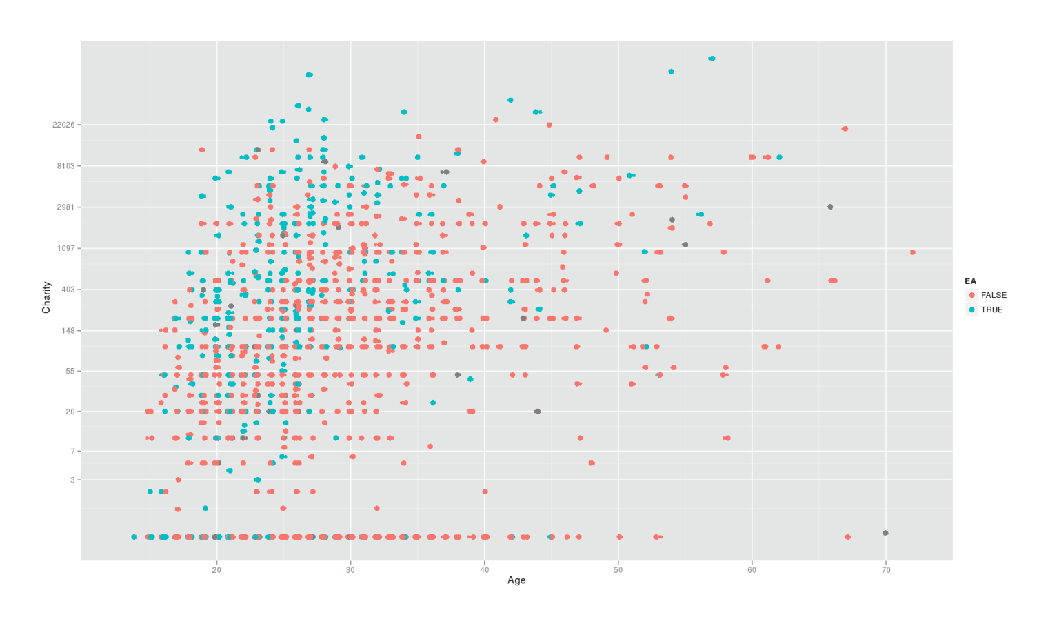
2013–201412ya LW surveyors’ reported donations over age, colored by self-identifying as EA
qplot(jitter(Age), jitter(CharityLog,a=0.1), color=EffectiveAltruism,
      data=na.omit(subset(survey, select=c(Age, CharityLog, EffectiveAltruism))), alpha=I(0.5)) +
 labs(x = "Age", y = "Charity", color ="EA") +  geom_point(size=I(3)) + stat_smooth()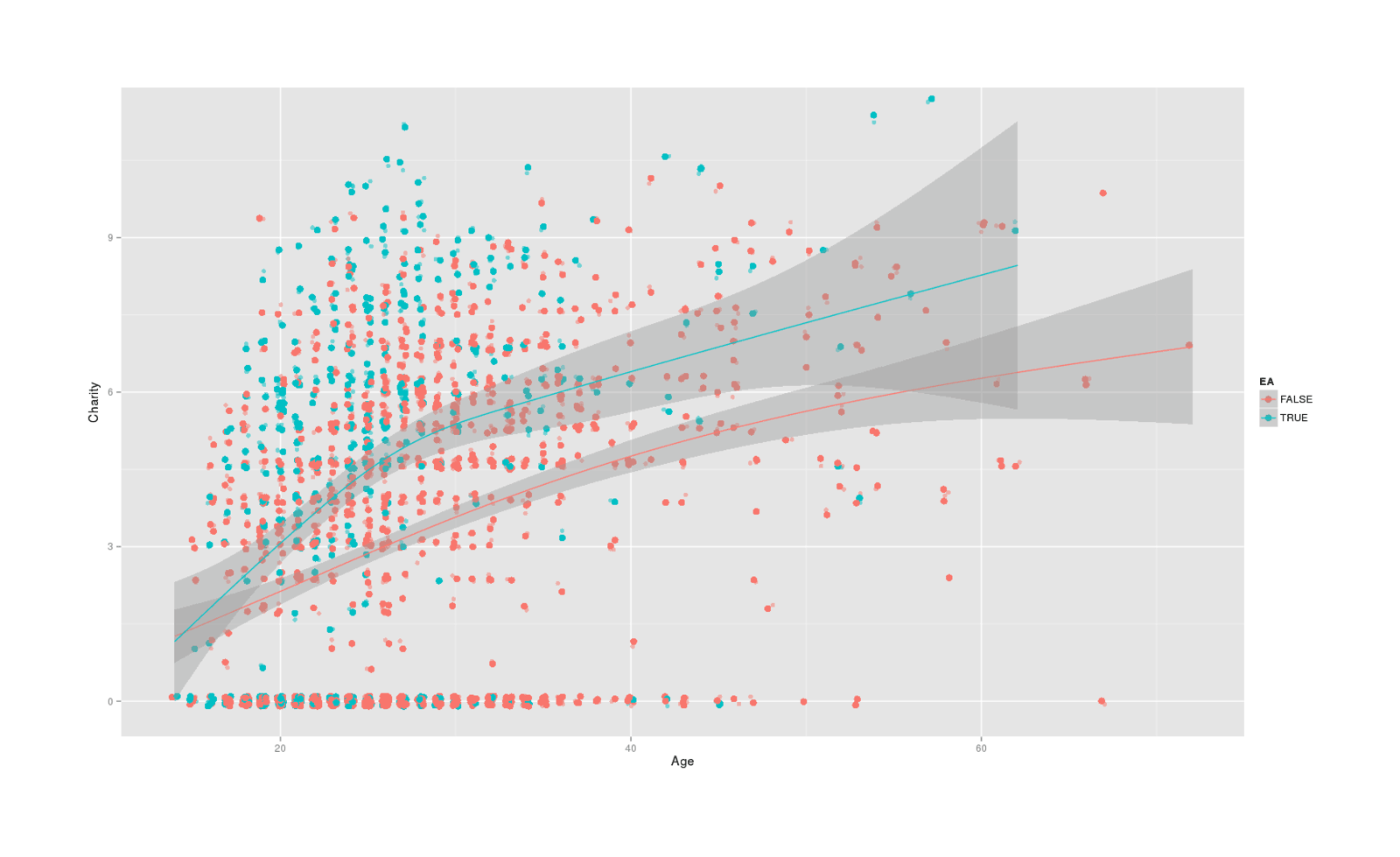
Reported donations over age, colored by EA; with GAM-smoothed curves of EA vs non-EA age-charity trend
# you might think that we can't treat Age linearly because this looks like a quadratic or
# logarithm, but when I fitted some curves, charity donations did not seem to flatten out
# appropriately, and the GAM/loess wiggly-but-increasing line seems like a better summary.
# Try looking at the asymptotes & quadratics split by group as follows:
#
## n1 <- nls(CharityLog ~ SSasymp(as.integer(Age), Asym, r0, lrc),
##            data=survey[survey$EffectiveAltruism,], start=list(Asym=6.88, r0=-4, lrc=-3))
## n2 <- nls(CharityLog ~ SSasymp(as.integer(Age), Asym, r0, lrc),
##            data=survey[!survey$EffectiveAltruism,], start=list(Asym=6.88, r0=-4, lrc=-3))
## with(survey, plot(Age, CharityLog))
## points(predict(n1, newdata=data.frame(Age=0:70)), col="blue")
## points(predict(n2, newdata=data.frame(Age=0:70)), col="red")
##
## l1 <- lm(CharityLog ~ Age + I(Age^2), data=survey[survey$EffectiveAltruism,])
## l2 <- lm(CharityLog ~ Age + I(Age^2), data=survey[!survey$EffectiveAltruism,])
## with(survey, plot(Age, CharityLog));
## points(predict(l1, newdata=data.frame(Age=0:70)), col="blue")
## points(predict(l2, newdata=data.frame(Age=0:70)), col="red")
#
# So I will treat Age as a linear/additive sort of thing.
# for the regression, we want to combine EffectiveAltruism/EffectiveAltruism2 into a single measure, EA, so
# a latent variable in a SEM; then we use EA plus the other covariates to estimate the CharityLog.
library(lavaan)
model1 <- " # estimate EA latent variable:
EA =~ EffectiveAltruism + EffectiveAltruism2
CharityLog ~ EA + Age + IncomeLog + Year +
# Degree dummies:
None + Highschool + twoyeardegree + Bachelors + Masters + Other +
MDJDotherprofessionaldegree + PhD. +
# WorkStatus dummies:
Independentlywealthy + Governmentwork + Forprofitwork +
Selfemployed + Nonprofitwork + Academicsontheteachingside +
Student + Homemaker + Unemployed
"
fit1 <- sem(model = model1, missing="fiml", data = survey); summary(fit1)
## lavaan (0.5-16) converged normally after 197 iterations
##
## Number of observations 2253
##
## Number of missing patterns 22
##
## Estimator ML
## Minimum Function Test Statistic 90.659
## Degrees of freedom 40
## P-value (Chi-square) 0.000
##
## Parameter estimates:
##
## Information Observed
## Standard Errors Standard
##
## Estimate Std.err Z-value P(>|z|)
## Latent variables:
## EA =~
## EffectvAltrsm 1.000
## EffctvAltrsm2 0.355 0.123 2.878 0.004
##
## Regressions:
## CharityLog ~
## EA 1.807 0.621 2.910 0.004
## Age 0.085 0.009 9.527 0.000
## IncomeLog 0.241 0.023 10.468 0.000
## Year 0.319 0.157 2.024 0.043
## None -1.688 2.079 -0.812 0.417
## Highschool -1.923 2.059 -0.934 0.350
## twoyeardegree -1.686 2.081 -0.810 0.418
## Bachelors -1.784 2.050 -0.870 0.384
## Masters -2.007 2.060 -0.974 0.330
## Other -2.219 2.142 -1.036 0.300
## MDJDthrprfssn -1.298 2.095 -0.619 0.536
## PhD. -1.977 2.079 -0.951 0.341
## Indpndntlywlt 1.175 2.119 0.555 0.579
## Governmentwrk 1.183 1.969 0.601 0.548
## Forprofitwork 0.677 1.940 0.349 0.727
## Selfemployed 0.603 1.955 0.309 0.758
## Nonprofitwork 0.765 1.973 0.388 0.698
## Acdmcsnthtchn 1.087 1.970 0.551 0.581
## Student 0.879 1.941 0.453 0.650
## Homemaker 1.071 2.498 0.429 0.668
## Unemployed 0.606 1.956 0.310 0.757
##
## Intercepts:
## EffectvAltrsm 0.319 0.011 28.788 0.000
## EffctvAltrsm2 0.109 0.012 8.852 0.000
## CharityLog -0.284 0.737 -0.385 0.700
## EA 0.000
##
## Variances:
## EffectvAltrsm 0.050 0.056
## EffctvAltrsm2 0.064 0.008
## CharityLog 7.058 0.314
## EA 0.168 0.056
# simplify:
model2 <- " # estimate EA latent variable:
EA =~ EffectiveAltruism + EffectiveAltruism2
CharityLog ~ EA + Age + IncomeLog + Year
"
fit2 <- sem(model = model2, missing="fiml", data = survey); summary(fit2)
## lavaan (0.5-16) converged normally after 55 iterations
##
## Number of observations 2253
##
## Number of missing patterns 22
##
## Estimator ML
## Minimum Function Test Statistic 70.134
## Degrees of freedom 6
## P-value (Chi-square) 0.000
##
## Parameter estimates:
##
## Information Observed
## Standard Errors Standard
##
## Estimate Std.err Z-value P(>|z|)
## Latent variables:
## EA =~
## EffectvAltrsm 1.000
## EffctvAltrsm2 0.353 0.125 2.832 0.005
##
## Regressions:
## CharityLog ~
## EA 1.770 0.619 2.858 0.004
## Age 0.085 0.009 9.513 0.000
## IncomeLog 0.241 0.023 10.550 0.000
## Year 0.329 0.156 2.114 0.035
##
## Intercepts:
## EffectvAltrsm 0.319 0.011 28.788 0.000
## EffctvAltrsm2 0.109 0.012 8.854 0.000
## CharityLog -1.331 0.317 -4.201 0.000
## EA 0.000
##
## Variances:
## EffectvAltrsm 0.049 0.057
## EffctvAltrsm2 0.064 0.008
## CharityLog 7.111 0.314
## EA 0.169 0.058
# simplify even further:
summary(lm(CharityLog ~ EffectiveAltruism + EffectiveAltruism2 + Age + IncomeLog, data=survey))
## ...Residuals:
## Min 1Q Median 3Q Max
## -7.6813410 -1.7922422 0.3325694 1.8440610 6.5913961
##
## Coefficients:
## Estimate Std. Error t value Pr(>|t|)
## (Intercept) -2.06062203 0.57659518 -3.57378 0.00040242
## EffectiveAltruismTRUE 1.26761425 0.37515124 3.37894 0.00081163
## EffectiveAltruism2TRUE 0.03596335 0.54563991 0.06591 0.94748766
## Age 0.09411164 0.01869218 5.03481 7.7527e-07
## IncomeLog 0.32140793 0.04598392 6.98957 1.4511e-11
##
## Residual standard error: 2.652323 on 342 degrees of freedom
## (1906 observations deleted due to missingness)
## Multiple R-squared: 0.2569577, Adjusted R-squared: 0.2482672
## F-statistic: 29.56748 on 4 and 342 DF, p-value: < 2.2204e-16Note these increases are on a log-dollars scale.
Conclusion
In all the analyses, median donations are >$0, and EAers report donating more. There is also Yvain’s predicted correlation of age with donation amount.
That said, the increase for EA donations is not as large as I would have expected: the median donation is increased by something like ~$1-50, and the simplest regression estimate is a factor of natural-log +1.3 or exp(1.3) → 3, which is much more impressive but I am not confident in this holding up because the scatter-plots suggest that this may wind up being an increase in donations while young but there are hardly any old EAers to judge from, so the net increase in donations over time may wind up being minimal as EAers converge with non-EAers with age. (That is, it’s great that a 20yo donates $60 rather than $20 and EA views may be causing this increase, but if at age 50 that 20yo would be donating $50,000 whether or not he had ever encountered EA, then EA has not done much good in the end.)