3 magnesium self-experiments on magnesium l-threonate and magnesium citrate.
The elemental metal magnesium (Examine.com), like lithium or potassium (which didn’t help me & damaged my sleep), plays many biological roles and has an RDA for me of 400mg which is higher than I likely get (most people apparently get less, with 68% of American adults <RDA; and while I frequently eat oats, milk, peanut butter, and whole-wheat bread, I don’t eat many leafy greens and my tap water is very soft). The anecdotes are the usual positive effects: general benefits, life improvements, higher affect; the interesting bits are the claims that magnesium is anxiolytic and affects sleep (positively, if you don’t mind the increase in dreaming, which makes me wonder if the benefits ascribed to float tanks might not be due to absorbing magnesium via the Epsom salts which provide the buoyancy).
L-Threonate
There are a variety of substances to get magnesium from. Considerable enthusiasm for the new compound magnesium l-threonate was stirred by 2 small animal rat studies finding that magnesium l-threonate was able to increase magnesium levels in the brain and improve learning/memory tasks. (There are no published human trials as of October 2015, and evidence of publication bias, which I take as evidence against there being large effects in humans.) Animal studies mean very little, of course (see the appendix), but I thought it’d be interesting to try using l-threonate, so I bought the $40.68$302013 “Life Extension Neuro-Mag Magnesium L-Threonate with Calcium and Vitamin D3 (205g)”, which according to the LEF product page works out to ~60g of “Magtein™ magnesium L-threonate” and ~4.31g elemental magnesium inasmuch as LEF claims 2000mg of threonate powder provides 144mg elemental magnesium or a 14:1 ratio. (I don’t need the calcium or vitamin D3, but this was the only magnesium l-threonate on Amazon.) Experiment-wise, I’ll probably look at sleep metrics and Mnemosyne performance; I put off designing a blind self-experiment until after trying some.
The powder itself is quite bulky; the recommended dose to hit 200mg of absorbed magnesium leads to ~7g of powder (so capping will be difficult) and the container provides only 30 doses’ worth (or each dose costs $1.36$12013!). It’s described as lemon-flavored, and it is, but it’s sickly-sweet unpleasant and since it’s so much powder, takes half a glass of water to dissolve it entirely and wash it down. Subjectively, I notice nothing after taking it for a week. I may try a simple A-B-A analysis of sleep or Mnemosyne, but I’m not optimistic. And given the large expense of LEF’s “Magtein”, it’s probably a non-starter even if there seems to be an effect. For sleep effects, I will have to look at more reasonably priced magnesium sources.
One thing I did do was piggyback on my Noopept self-experiment: I blinded & randomized the Noopept for a real experiment, but simply made sure to vary the Magtein without worrying about blinding or randomizing it. (The powder is quite bulky.) The correlation the experiment turned in was an odds-ratio of 1.9; interesting and in the right direction (higher is better), but since the magnesium part wasn’t random or blind, not a causal result.
Citrate
Experiment 1
Encouraged by TruBrain’s magnesium & my magnesium l-threonate use, I design and run a blind random self-experiment to see whether magnesium citrate supplementation would improve my mood or productivity. I collected ~200 days of data at two dose levels. The analysis finds that the net effect was negative, but a more detailed look shows time-varying effects with a large initial benefit negated by an increasingly-negative effect. Combined with my expectations, the long half-life, and the higher-than-intended dosage, I infer that I overdosed on the magnesium. To verify this, I will be running a followup experiment with a much smaller dose.
The original magnesium l-threonate caused me no apparent problems by the time I finished off the powder and usage correlated with better days, further supporting the hypothesis that magnesium helps it. But l-threonate would be difficult to cap (and hence blind self-experiment) and is ruinously expensive on a per-dose basis. So I looked around for alternatives for the followup; one of the most common compounds suggested was the citrate form because it is reasonably well-absorbed and causes fewer digestive problems, so I could just take that. Magnesium oxide is widely available it looks cheap, but the absorption/bioavailability problem makes it unattractive: at a 3:5 ratio, an estimate of 4% absorption, a ZMA formulation of an impressive-sounding 500mg would be 500 × 3⁄5 × 0.04 = 12mg or a small fraction of RDAs for male adults like 400mg elemental. (Calcium shouldn’t be a problem since I get 220mg of calcium from my multivitamin and I enjoy dairy products daily.)
Finding an usable product on Amazon caused me some difficulties. I wanted a 500mg magnesium-citrate-only product at <$26.72$202014 for 120 doses, but I discovered most of the selection for “magnesium citrate” had sub-500mg doses, involved calcium citrate or other substances like zinc (not necessarily a bad thing, but would confound an experiment), were mostly magnesium oxide rather than citrate, or some still other problem. Ultimately I settled on Solgar’s 120x400mg magnesium citrate ($17.37$132014) as acceptable. (To compare with the bulkiness of the LEF vitamin D+l-threonate powder, the Office of Dietary Supplements says magnesium citrate is 16% magnesium, so to get 400mg of magnesium as claimed, would take 2.5g of material, rather than 7g for 200mg; even if l-threonate is absorbed 100% and citrate 50%, the citrate is ahead. The pills turn out to be wider and longer than my 00 pills; if I want to get them into my gel capsules, I have to crush them into fine powder. The powder from one pill turns out to take up 2 00 pills.)
My impression after the first two days (2 doses of 400mg each, one with breakfast & then lunch) was positive. I did not have the rumored digestion problems, and the first day went excellently: I was up until 1:30AM working and even then didn’t feel like going to bed—and I probably should have since I then slept abominably, which made the second day merely a good day. The third day I took none and it was an ordinary day. This is consistent with what I expected from the LEF l-threonate & TruBrain glycinate/lycinate, and so it is worth investigating with a self-experiment.
Experiment
The basic idea is to remedy a deficiency (not look for acute stimulant effects) and magnesium has a slow excretion rate1, so week-long blocks seem appropriate. I can reuse the same methodology as the lithium self-experiment. The response variables will be the usual mood/productivity self-rating and, since I was originally interested in magnesium for possible sleep quality improvements, a standardized score of sleep latency + # of awakenings + time spent awake (the same variable as my potassium sleep experiment).
Since each 400mg pill takes up 2 00 pills, that’s 4 gel caps a day to reach 800mg magnesium citrate (ie. 136mg elemental magnesium), or 224 gel caps (2x120) for the first batch of Solgar magnesium pills. Turning the Solgar tablets into gel capsules was difficult enough that I switched to NOW Food’s 227g magnesium citrate powder for the second batch.
Power
Reusing the magnesium correlation from the first Noopept self-experiment and using the t-test as an approximation
pwr.t.test(d = (0.27 / sd(npt$MP)), power = 0.8, type="paired", alternative="greater")
# Paired t test power calculation
#
# n = 50.61
# ...
50 pairs of active/placebos or 100 days. With 120 tablets and 4 tablets used up, that leaves me 58 doses. That might seem adequate except the paired t-test approximation is overly-optimistic, and I also expect the non-randomized non-blinded correlation is too high which means that is overly-optimistic as well. The power would be lower than I’d prefer. I decided to simply order another bottle of Solgar’s & double the sample size to be safe.
Is 200 enough? There are no canned power functions for the ordinal logistic regression I would be using, so the standard advice is to estimate power by simulation: generating thousands of new datasets where we know by construction that the binary magnesium variable increases MP by 0.27 (such as by bootstrapping the original Noopept experiment’s data), and seeing how often in this collection the cutoff of statistical-significance is passed when the usual analysis is done (background: CrossValidated or “Power Analysis and Sample Size Estimation using Bootstrap”). In this case, we leave alpha at 0.05, reuse the Noopept experiment’s data with its Magtein correlation, and ask for the power when n = 200
library(boot)
library(rms)
npt <- read.csv("https://gwern.net/doc/nootropic/quantified-self/2013-gwern-noopept.csv")
n <- 200
magteinPower <- function(dt, indices) {
    d <- dt[sample(nrow(dt), n, replace=TRUE), ] # new dataset, possibly larger than the original
    lmodel <- lrm(MP ~ Noopept + Magtein, data = d)
    return(anova(lmodel)[8])
}
bs <- boot(data=npt, statistic=magteinPower, R=100000, parallel="multicore", ncpus=4)
alpha <- 0.05
print(sum(bs$t<=alpha)/length(bs$t))
# [1] 0.7132
So the power will be ~71%.
Data
-
27 August–2 September: 0
3 September–9 September: 1
-
10 September–15 September: 0
16 September–21 September: 1
-
22 September–28 September: 0
29 September–5 October: 1
-
6 October–12 October: 0
13 October–19 October: 1
-
21 October–27 October: 1
28 October–2 November: 0
-
5 November–11 November: 1 (skipped 3/4 November)
During 11 November, I accidentally unblinded myself while cleaning my room. Hence, I refilled the active jar and began a fresh pair of blocks.
-
12–17 November: 0
18–24 November: 1
-
25–29 November: 0; on 30 November, I again unblinded myself and started over later.
-
2–8 December: 1
9–15 December: 0
-
16–17 December: 0
18–19 December: 1
At this point, I discovered I had run out of magnesium pills and had forgotten to order the magnesium citrate powder I’d intended to. I still had a lot of Noopept pills for the concurrently running second Noopept self-experiment, but since I wanted to wrap up some other experiments with a big analysis at the end of the year, I decided to halt and resume in January 2014.
-
25–2014-01-31: 0
1 February–7 February: 1
For this batch, I tried out “NOW Foods Magnesium Citrate Powder” ($9.35$72014 for 227g); the powder was still a bit sticky but much easier to work with than the Solgar pills, and the 227g made 249 gel capsule pills. The package estimates 119 serving of 315mg elemental magnesium, so a ratio of 0.315g magnesium for 1.9g magnesium citrate, implying that each gel cap pill then contains 0.152g magnesium ((119×315) ⁄ 249 = 150) and since I want a total dose of 0.8g, I need 5 of the gel cap pills a day or 35 per block.
-
9–15 February: 1 (skipped 8 February)
16–22 February: 0
-
23–1 March: 1
2–8 March: 0
-
9–15 March: 1
16–22 March: 0
-
23–29 March: 0
30 March–5 April: 1
-
6–12 April: 0
13–19 April: 1
-
20–26 April: 0
27 April–3 May: 1
Subjectively, I have no particular comments, other than that (like the threonate), I noticed no diarrhea.
Analysis
Some prep:
magnesium <- read.csv("magnesium.csv")
mp <- read.csv("~/selfexperiment/mp.csv")
mp$MP <- as.integer(as.character(mp$MP))
rm(magnesium$MP)
magnesium <- merge(mp, magnesium, all=TRUE)
write.csv(magnesium, file="magnesium.csv", row.names=FALSE)
The basic question: did the magnesium citrate increase MP?
magnesium <- read.csv("https://gwern.net/doc/nootropic/quantified-self/2013-2014-magnesium.csv")
summary(lm(MP ~ Magnesium.citrate, data=magnesium))
# Coefficients:
#                    Estimate Std. Error t value Pr(>|t|)
# (Intercept)        3.276515   0.056677   57.81   <2e-16
# Magnesium.citrate -0.000543   0.000144   -3.79    2e-04
#
# Residual standard error: 0.671 on 206 degrees of freedom
#   (678 observations deleted due to missingness)
# Multiple R-squared:  0.065,   Adjusted R-squared:  0.0605
# F-statistic: 14.3 on 1 and 206 DF,  p-value: 0.000201
mean(-0.000543 * c(136, 800))
# [1] -0.2541
The initial results are a shock: the mean effect of the magnesium citrate comes in at almost the exact same magnitude (-0.25) as had been estimated for the Magtein back in the original Noopept analysis (0.26), except the estimated average effect is negative, as in, the magnesium citrate was harmful, and statistically-significantly so. Huh?
This was so unexpected that I wondered if I had somehow accidentally put the magnesium pills into the placebo pill baggie or had swapped values while typing up the data into a spreadsheet, and checked into that. The spreadsheet accorded with the log above, which rules out data entry mistakes; and looking over the log, I discovered that some earlier slip-ups were able to rule out the pill-swap: I had carelessly put in some placebo pills made using rice, in order to get rid of them, and that led to me being unblinded twice before I became irritated enough to pick them all out of the bag of placebos—but how could that happen if I had swapped the groups of pills?
So I began looking further into the data to see just what had happened (perhaps bad luck on a few days?), and turned to a plot:
library(ggplot2)
magnesium$Date <- as.Date(magnesium$Date)
with(magnesium[559:nrow(magnesium),],
qplot(Date, MP, color=as.factor(Magnesium.citrate), legend="Magnesium citrate", size=I(7)) +
       scale_colour_manual(values=c("gray49", "red1", "red3"), name = "Magnesium"))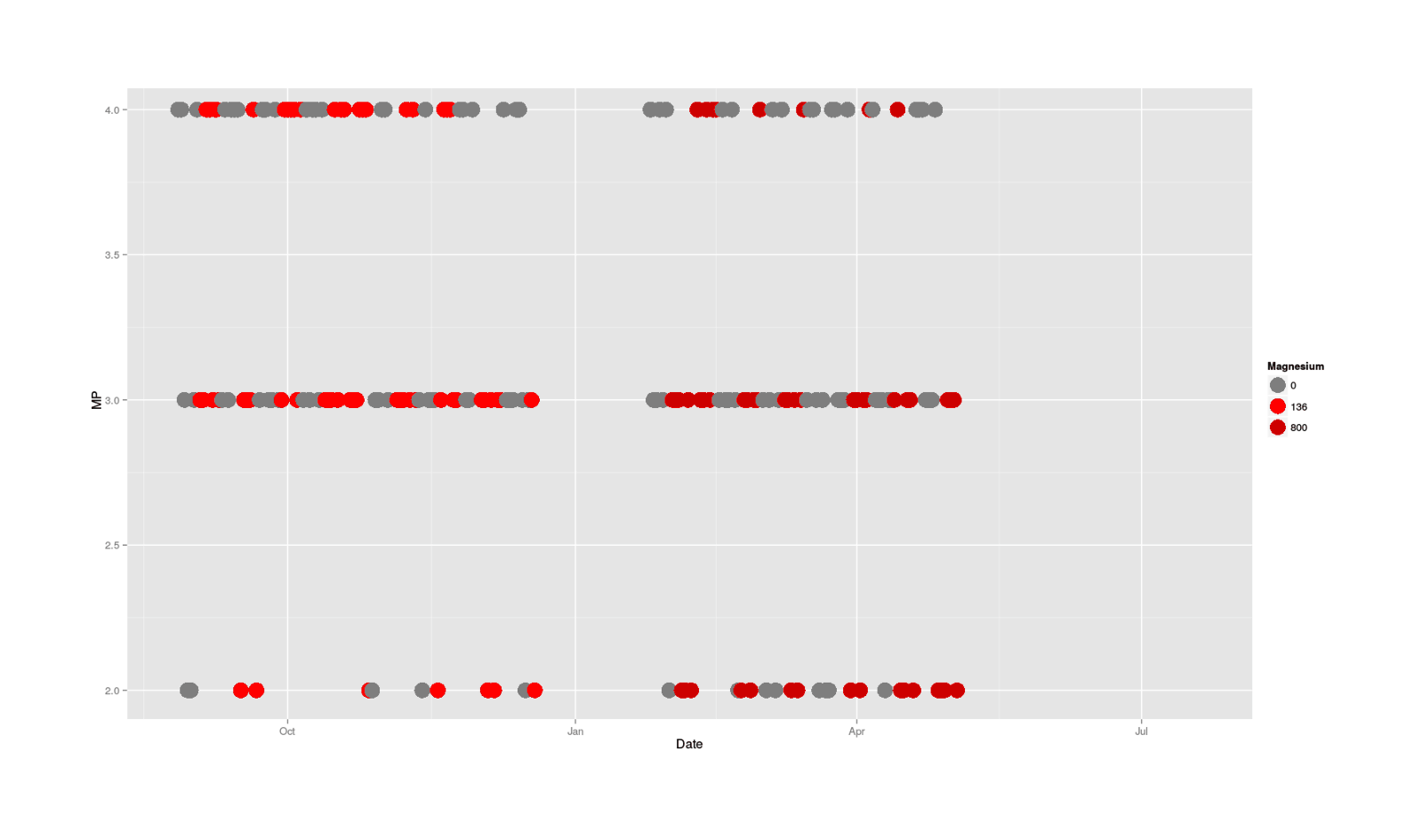
One thing I notice looking at the data is that the red magnesium-free days seem to dominate the upper ranks towards the end, and blues appear mostly at the bottom, although this is a little hard to see because good days in general start to become sparse towards the end. Now, why would days start to be worse towards the end, and magnesium-dose days in particular?
The grim surmise is: an accumulating overdose—no immediate acute effect, but the magnesium builds up, dragging down all days, but especially magnesium-dose days. The generally recognized symptoms of hypermagnesemia don’t include effect on mood or cognition, aside from “muscle weakness, confusion, and decreased reflexes…poor appetite that does not improve”, but it seems plausible that below medically-recognizable levels of distress like hypermagnesemia might still cause mental changes, and I wouldn’t expect any psychological research to have been done on this topic.
A picture is worth a thousand words, particularly in this case where there seems to be temporal effects, different trends for the conditions, and general confusion. So, I drag up 2.5 years of MP data (for context), plot all the data, color by magnesium/non-magnesium, and fit different LOESS lines to each as a sort of smoothed average (since categorical data is hard to interpret as a bunch of dots), which yields:
magnesium[is.na(magnesium$Magnesium.citrate),]$Magnesium.citrate <- -1
ggplot(data = magnesium, aes(x=Date, y=MP, col=as.factor(magnesium$Magnesium.citrate))) +
 geom_point(size=I(4)) +
 stat_smooth() +
 scale_colour_manual(values=c("gray49", "grey35", "red1", "red3" ),
                     name = "Magnesium")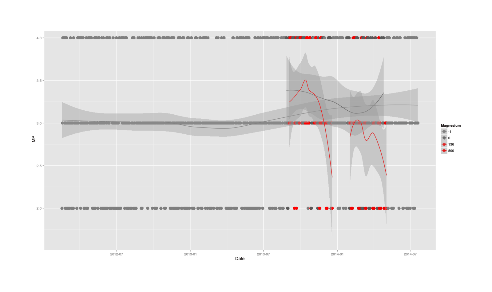
That really says it all: there’s an initial spike in MP, which reads like the promised stimulative effects possibly due to fixing a deficiency (a spike which doesn’t seem to have any counterparts in the previous history of MP), followed by a drastic plunge in the magnesium days but not so much the control days (indicating an acute effect when overloaded with magnesium), a partial recovery during the non-experimental Christmas break, another plunge, and finally recovery after the experiment has ended.
We can verify the negative correlation with the date & an interaction between magnesium and the date; I don’t know whether to treat the magnesium dose as a linear, categorical, or logical, so I’ll try all of them:
magnesium <- read.csv("https://gwern.net/doc/nootropic/quantified-self/2013-2014-magnesium.csv")
magnesium$Date <- as.integer(magnesium$Date)
slm <- step(lm(MP ~ Magnesium.citrate * as.logical(Magnesium.citrate) *
                    as.factor(Magnesium.citrate) * Date * Noopept, data=magnesium))
# MP ~ as.logical(Magnesium.citrate) + Date + as.logical(Magnesium.citrate):Date
summary(slm)
# Coefficients:
#                                         Estimate Std. Error t value Pr(>|t|)
# (Intercept)                             3.942875   0.571166    6.90  6.3e-11
# as.logical(Magnesium.citrate)TRUE       1.217860   0.806212    1.51    0.132
# Date                                   -0.000992   0.000830   -1.20    0.233
# as.logical(Magnesium.citrate)TRUE:Date -0.002105   0.001173   -1.79    0.074
#
# Residual standard error: 0.664 on 204 degrees of freedom
#   (678 observations deleted due to missingness)
# Multiple R-squared:  0.0933,  Adjusted R-squared:  0.08
# F-statistic:    7 on 3 and 204 DF,  p-value: 0.000167
As feared and consistent with the accumulating overdose hypothesis, scores decrease over time and they decrease if magnesium is used that day. (The interaction isn’t statistically-significant, but I am not surprised: I powered this self-experiment to detect one main effect, not two main effects and an interaction.)
But at least initially, the magnesium seemed to be remarkably useful. The crossover point, using this linear model, would have been somewhere around 20 days of the early small magnesium doses:
## Extract estimated MP for continuous small magnesium dosing, then for no magnesium dosing;
## compare them pair-wise to see which is bigger, and count how many days favor magnesium dosing.
with(magnesium[!is.na(magnesium$Magnesium.citrate),], sum(predict(slm, newdata=data.frame(Date=Date, Magnesium.citrate=136)) >
                                                          predict(slm, newdata=data.frame(Date=Date, Magnesium.citrate=0))))
# [1] 20
The final question is: since I was taking an overdose, how did I mess up? I thought I was making sure I got at least the right RDA of elemental magnesium by aiming for 800mg of elemental magnesium and carefully converting from raw powder weight. So I went back to the original references, and scrutinizing them closely, they really were talking about elemental magnesium and indicating I should be getting 400mg elemental a day, but I did notice something: I got the dose wrong for the Solgar pills, it wasn’t 800mg elemental, it was 800mg of citrate—I misread the label. So I went from taking ~130mg of elemental magnesium in the first period to ~800mg in the second; I don’t think it is an accident that the second period seems to have been much worse (between the plot and the time trend).
I find this very troubling. The magnesium supplementation was harmful enough to do a lot of cumulative damage over the months involved (I could have done a lot of writing September 2013–June 2014), but not so blatantly harmful enough as to be noticeable without a randomized blind self-experiment or at least systematic data collection—neither of which are common among people who would be supplementing magnesium I would much prefer it if my magnesium overdose had come with visible harm (such as waking up in the middle of the night after a nightmare soaked in sweat), since then I’d know quickly and surely, as would anyone else taking magnesium. But the harm I observed in my data? For all I know, that could be affecting every user of magnesium supplements! How would we know otherwise?
Sleep
I reused the magnesium data with my Zeo data and looked at the effects. The result were ambiguous: only a few effects survive multiple correction, which were a mix of good and bad ones, and I would guess that some of the bad effects are due to too much magnesium (although there is no time trend as blatant).
Conclusion
The interpretation which seems to best resolve everything I know about magnesium with the data from my experiment is that magnesium supplementation does indeed help me a large amount, but I was taking way too much.
Experiment 2
This is not 100% clear from the data and just blindly using a plausible amount carries the risk of the negative effects, so I intend to run another large experiment. I will reuse the “NOW Foods Magnesium Citrate Powder”, but this time, I will use longer blocks (to make cumulative overdosing more evident) and try to avoid any doses >150mg of elemental magnesium.
I spent 2.5 hours making gel capsules:
-
10x24 Bisquick placebo
-
10x24 magnesium citrate
-
480 total
The powder totals 227g of magnesium citrate, hence there is ~0.945g per magnesium citrate pill. The nutritional information states that it contains 119 servings of 0.315g magnesium elemental = 37.485g elemental, as expected, and so likewise there is 0.156g elemental magnesium per pill. This is the same dosage as the second half of the first magnesium citrate experiment (249 gel capsules there, 240 here), where the overdose effect seemed to also happen; so to avoid the overdosage, I will take one pill every other day to halve the dose to an average of ~0.078g/78mg elemental per day (piggybacking on the morning-caffeine experiment to make compliance easier).
At 1 pill every other day, 14 doses, so pairs of 28-day blocks. The total time to use up all pills will then be ~960 days; this is a long time and excessively-powered, so I may stop early or possibly do a sequential analysis.
The benefit of sequential analysis here is being able to stop early, conserving pills, and letting me test another dosage: if I see another pattern of initial benefits followed by decline, I can then try cutting the dose by taking one pill every 3 days; or, if there is a benefit and no decline, then I can try tweaking the dose up a bit (maybe 3 days out of 5?). Since I don’t have a good idea what dose I want and the optimal dose seems like it could be valuable (and the wrong dose harmful!), I can’t afford to spend a lot of time on a single definitive experiment.
Power
Since I didn’t take any 78mg elemental doses and the effects were time-varying, it’s more difficult to estimate the expected effect-size and hence power.
If I assume that the coefficient of +1.22 for as.logical(Magnesium.citrate)TRUE’s effect on MP in the previous analysis represents the true causal effect of 0.156g elemental magnesium without any overdose involved and that magnesium would have a linear increase (up until overdose), then one might argue that optimistically 0.078 would cause an increase of ~0.61. Or one could eyeball the graph and note that the LOESS lines look like at the magnesium peak improved by <+0.5 over the long-run baseline of ~3 Then one could do a power estimate with those 2 estimates.
## _d_:
0.61 / sd(magnesium$MP, na.rm=TRUE)
# [1] 0.83795623
power.t.test(n = 480, delta = 0.83)
#  Two-sample t test power calculation
#
#            n = 480
#        delta = 0.83
#           sd = 1
#    sig.level = 011.05
#        power = 1
power.t.test(delta = 0.83, power = 0.9)
# Two-sample t test power calculation
#
#          n = 31.4970227
#      delta = 0.83
#         sd = 1
#  sig.level = 0.05
#      power = 0.9
0.5 / sd(magnesium$MP, na.rm=TRUE)
# [1] 0.686849369
power.t.test(delta = 0.68, power = 0.8)
# Two-sample t test power calculation
#
#          n = 34.9352817
power.t.test(delta = 0.5, power = 0.8)
# Two-sample t test power calculation
#
#          n = 63.7657637
Power considerations suggest I could probably terminate after 4 months
Data
-
29 August–2014-09-27: 0
28 September–2 November: 1
-
3 November–4 December: 0
5 December–2015-01-11: 1
-
12 January–18 February: 0
19 February–5 March: 1 (ended block early so I could have complete data for the LLLT experiment’s analysis)
-
6 March–4 April: 1
5 April–10 May: 0
-
11 May–12 June: 0
13 June–15 July: 1
-
16 July–6 September: 1
Thought I was done with both blocks so I unblinded myself, only to discover I wasn’t. Oops.
-
7 September–7 November: 1 (skipped over half a month due to long trip)
8 November–2016-01-08: 0
-
4 March–28 April: 0
29 April:–25 May: 1
-
1 June–28 June: 1
29 June–26 July: 0
-
27 July–24 August: 1
25 August–21 September: 0
-
22 September–16 October: 1
17 October–10 November: 0
Analysis
Conclusion
78mg, every other day
Prep
mp <- na.omit(read.csv("~/selfexperiment/mp.csv", colClasses=c("Date", "integer")))
magnesium2 <- read.csv("~/2016-10-10-magnesium-second.csv", header=TRUE, colClasses=c("Date", "integer", "integer"))

magnesium <- merge(magnesium2, mp)

write.csv(magnesium, file="~/wiki/doc/nootropic/quantified-self/2016-10-10-magnesium-second.csv", row.names=FALSE)
Descriptive
magnesium <- read.csv("~/wiki/doc/nootropic/quantified-self/2016-10-10-magnesium-second.csv",
               colClasses=c("Date", "integer", "integer", "integer", "numeric", "numeric", "numeric"))
library(skimr)
skim(magnesium)
# Skim summary statistics
#  n obs: 767
#  n variables: 7
#
# Variable type: Date
#  variable missing complete   n        min        max     median n_unique
#      Date       0      767 767 2014-08-29 2016-11-10 2015-09-16      767
#
# Variable type: integer
#      variable missing complete   n  mean    sd p0 p25 p50 p75 p100     hist
#          Dose       0      767 767 18.41 33.14  0   0   0   0   78 ▇▁▁▁▁▁▁▂
#  Experimental      56      711 767  0.5   0.5   0   0   1   1    1 ▇▁▁▁▁▁▁▇
#            MP       0      767 767  3.2   0.64  1   3   3   4    5 ▁▂▁▇▁▅▁▁
#
# Variable type: numeric
#              variable missing complete   n  mean    sd p0     p25   p50  p75 p100     hist
#       Dose.cumulative       0      767 767 1.21  0.56   0 0.85    1.21  1.56 2.42 ▂▃▅▇▇▆▂▃
#  Dose.cumulative.fast       0      767 767 0.059 0.061  0 5.8e-07 0.033 0.1  0.15 ▇▁▁▁▁▃▁▃
#  Dose.cumulative.slow       0      767 767 1.15  0.54   0 0.81    1.16  1.47 2.27 ▂▃▅▇▇▆▂▃

library(ggplot2)

magnesiumTmp[is.na(magnesiumTmp$Experimental),]$Experimental <- 0

with(magnesiumTmp, qplot(Date, MP, color=as.logical(Experimental), legend="Magnesium citrate") +
    scale_colour_manual(values=c("gray49", "red1"), name = "Magnesium") + stat_smooth())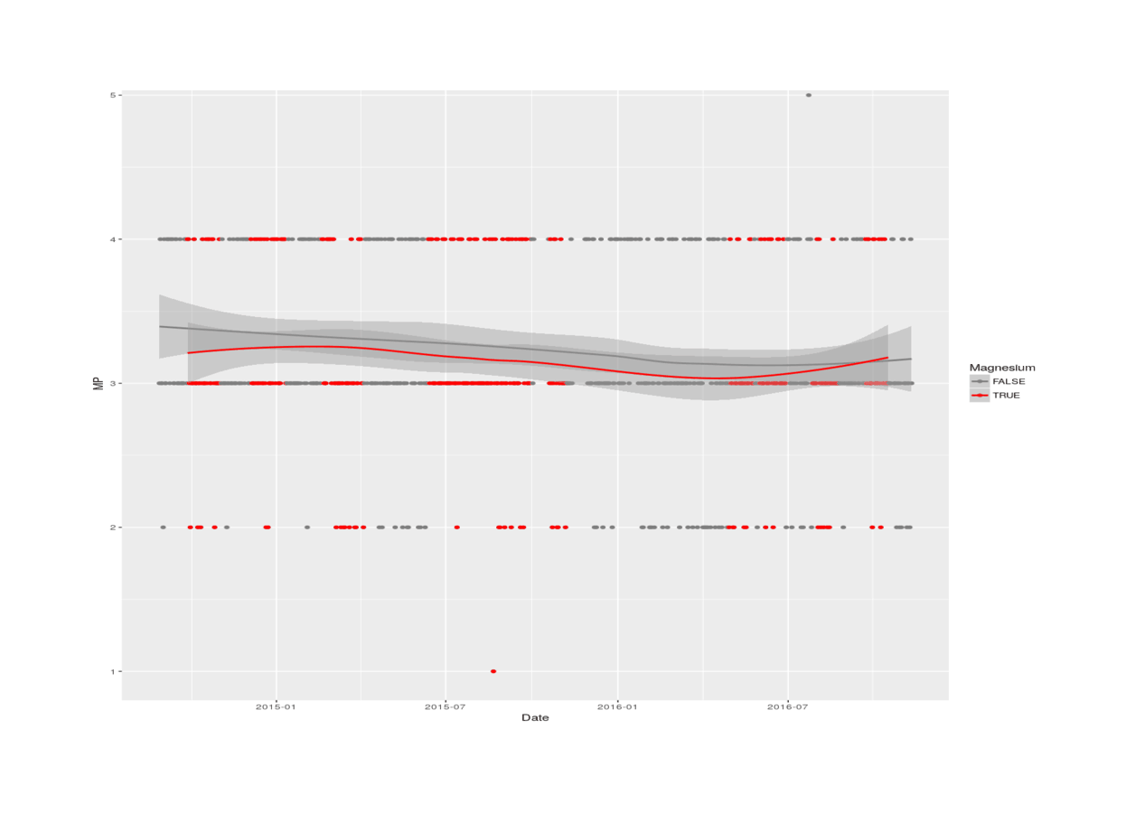
Testing
wilcox.test(MP ~ Experimental, data=magnesium)
#
#   Wilcoxon rank sum test with continuity correction
#
# data:  MP by Experimental
# W = 66897, p-value = 0.125959
# alternative hypothesis: true location shift is not equal to 0
summary(lm(MP ~ Date + Experimental, data=magnesium))
# ...Residuals:
#       Min        1Q    Median        3Q       Max
# -2.172324 -0.269037 -0.164076  0.714138  1.855738
#
# Coefficients:
#                  Estimate   Std. Error  t value   Pr(>|t|)
# (Intercept)   8.33930e+00  1.61701e+00  5.15722 3.2567e-07
# Date         -3.05501e-04  9.67501e-05 -3.15763  0.0016581
# Experimental -7.48915e-02  4.71081e-02 -1.58978  0.1123307
#
# Residual standard error: 0.627593 on 708 degrees of freedom
#   (56 observations deleted due to missingness)
# Multiple R-squared:  0.0168461,   Adjusted R-squared:  0.0140689
# F-statistic: 6.06572 on 2 and 708 DF,  p-value: 0.00244347

magnesium$Date.int <- as.integer(magnesium$Date)
library(brms)
## reasonably informative prior:
magnesium$Magnesium.citrate <- 0
b <- brm(MP ~ Date.int + I(Dose + Magnesium.citrate), prior=c(prior(normal(0,0.1/78), "b")),
          autocor=cor_arma(~1, p=0, q=1),
          iter=10000, chains=30, cores=30, data=magnesium); summary(b); fixef(b)
# Correlation Structures:
#       Estimate Est.Error l-95% CI u-95% CI Eff.Sample Rhat
# ma[1]     0.15      0.04     0.07     0.22      84215 1.00
#
# Population-Level Effects:
#                         Estimate Est.Error l-95% CI u-95% CI Eff.Sample Rhat
# Intercept                   8.19      1.83     4.58    11.76     150000 1.00
# Date.int                   -0.00      0.00    -0.00    -0.00     150000 1.00
# IDosePMagnesium.citrate    -0.00      0.00    -0.00     0.00     150000 1.00
#
# Family Specific Parameters:
#       Estimate Est.Error l-95% CI u-95% CI Eff.Sample Rhat
# sigma     0.63      0.02     0.60     0.66      83059 1.00
#                                Estimate      Est.Error            Q2.5           Q97.5
# Intercept                8.187500103687 1.825404749366  4.581534432199  1.17586125e+01
# Date.int                -0.000297324482 0.000109197301 -0.000511038825 -8.14888755e-05
# IDosePMagnesium.citrate -0.000928834462 0.000571607891 -0.002050468458  1.87187142e-04
mean(fixef(b, summary=FALSE)[,3] < 0)
# [1] 0.94834
The standard binary test with a linear date trend indicates high probability of harm as before, and the estimated per-mg effect size of the halved (78mg) dose is similar to the original magnesium citrate per-mg effect size: the original estimate was -0.0005/mg; and the new is -0.0009/mg; so, similar, and actually higher (but well within the two estimates’ combined sampling error).
Unsurprisingly, combining the two experiments into a single analysis yields an intermediate effect size of -0.0006/mg (95% credible interval, -0.0008 to -0.0003) with P = 1 that it’s negative:
magnesium1 <- read.csv("https://gwern.net/doc/nootropic/quantified-self/2013-2014-magnesium.csv", colClasses=c("Date", rep("numeric", 4)))
magnesiumAll <- merge(magnesium, magnesium1, all=TRUE)
magnesiumAll$Date.int <- as.integer(magnesiumAll$Date)

magnesiumAllClean <- subset(magnesiumAll, select=c(Date, Date.int, MP, Experimental, Magnesium.citrate, Dose))
magnesiumAllClean <- magnesiumAllClean[!is.na(magnesiumAllClean$Dose) | !is.na(magnesiumAllClean$Magnesium.citrate),]
magnesiumAllClean[is.na(magnesiumAllClean)] <- 0

ba <- brm(MP ~ Date.int + I(Dose + Magnesium.citrate), prior=c(prior(normal(0,0.1/78), "b")),
          autocor=cor_arma(~1, p=0, q=1),
          iter=10000, chains=30, cores=30, data=magnesiumAllClean); summary(ba)
# Correlation Structures:
#       Estimate Est.Error l-95% CI u-95% CI Eff.Sample Rhat
# ma[1]     0.14      0.03     0.08     0.20      84642 1.00
#
# Population-Level Effects:
#                         Estimate Est.Error l-95% CI u-95% CI Eff.Sample Rhat
# Intercept                   6.53      1.21     4.16     8.89     150000 1.00
# Date.int                   -0.00      0.00    -0.00    -0.00     150000 1.00
# IDosePMagnesium.citrate    -0.00      0.00    -0.00    -0.00     150000 1.00
#
# Family Specific Parameters:
#       Estimate Est.Error l-95% CI u-95% CI Eff.Sample Rhat
# sigma     0.64      0.01     0.61     0.67      88110 1.00
#
# Samples were drawn using sampling(NUTS). For each parameter, Eff.Sample
# is a crude measure of effective sample size, and Rhat is the potential
# scale reduction factor on split chains (at convergence, Rhat = 1).
#                                Estimate      Est.Error           Q2.5           Q97.5
# Intercept                6.528906256390 1.20706045e+00  4.15836502039  8.89383946e+00
# Date.int                -0.000199023324 7.26410825e-05 -0.00034141518 -5.62550961e-05
# IDosePMagnesium.citrate -0.000616714063 1.36473721e-04 -0.00088489562 -3.49705762e-04
mean(fixef(ba, summary=FALSE)[,3] < 0)
# [1] 0.999986667
## so -0.0006 (-0.0008 - -0.0003) / mg, P=1
So the original result is not anomalous and is confirmed by the followup.
This is a disappointing finding on several levels: from a biological perspective, magnesium is a vital micronutrient and deficiency expected and getting a result of harm makes me question my methods & results; from a practical perspective, it means that in addition to the considerable work required to set up & run the self-experiments, I inflicted a nontrivial level of harm on myself (-0.06 on >1 year’s worth of days); and from a decision perspective, this result is, ex post, worthless, as my default decision is to not supplement magnesium and the additional information doesn’t change my decision and so has a VoI of zero (only somewhat ameliorated by the possibility that the results will be of interest or use to readers).
What might explain this harm? After thinking about the results some more, I have two suggestions:
-
Electrolyte Imbalance: I recall that there is another related supplement where my randomized blinded self-experiment found harm despite general reports of benefits and deficiencies: potassium.
Potassium is much like magnesium/sodium/calcium in being a metal and electrolyte heavily used by the nervous system and often supplemented for activities like sports. Could supplementing potassium and then magnesium, separately, have been causing electrolyte imbalance? This would elegantly resolve both findings of harm and explain why others find benefits (perhaps they had higher baseline levels of the necessary co-electrolytes, or were supplementing them simultaneously). Thiamine has also been suggested as a possible cofactor used up by magnesium supplementation.
In that case, the solution is simple: do some reading to find out if any optimal ratios have been measured yet, or simply take a common-sized dose of both potassium & magnesium (and perhaps sodium too—I am pretty sure I get more than enough calcium because I consume so much dairy, but I am not sure about sodium since I cook almost all my food & use little salt by default as I grew up in a low-sodium home & find even a little salt to be more than enough flavoring). There might be something useful in blood test panels too. Figuring out the right dose might be tricky, as overdoses can produce issues like milk-alkali syndrome.
Given the established harm, I would have to run yet a third self-experiment, one long enough to be able to rule out even a small harm and certify long-term use (which has potentially high regret).
-
Overdose: as mentioned in the first experiment, the fact that the harm seems like it increases over time is suspicious. This shows up less in the second one, but that uses a smaller dose and has longer & more breaks, so that might be why.
If it’s a cumulative overdose, since magnesium has a long half-life, modeling the hypothetical cumulative doses each day should offer some insight. If there turns out to be
No additional experimentation is needed, since the doses & dose schedule is known and there ought to be enough variation in sums to analyse. So I can do some exploratory analyses of this possibility.
Modeling Cumulative Dose
To model the possibility of overdose, I can take the existing data’s schedule of doses and use a magnesium half-life formula to calculate the increase in magnesium load each day over an assumed baseline of 0mg. Then regress as before, but on the total magnesium load, both linear and quadratic (for the dose-response curve).
So what’s the actual half-life of a magnesium supplement, besides “long”?
“Magnesium Basics” cites on the topic just the paper 1966, “Mg28 kinetics in man”. They trace magnesium in humans and fit to the data a rather complex multi-compartment model with several small (15% of total magnesium) fast-exchanging reservoirs of magnesium and a few large slow-exchanging reservoirs (the other 85%), all of which turnover and connect with each other at different rates. This would be unmanageable but they do suggest a simplified two-compartment model:
Most often the data have been treated with the assumption that each exponential function represented a discrete magnesium compartment with independent rates of turnover. On the basis of such analyses applied to urinary Mg28 specific activity curves, Silver et al (21) defined three exchanging magnesium compartments in man with half-times of 35 hr, 3 hr, and 1 hr, respectively…Zumoff (23) analyzing curves in normal subjects again described three components with half-lives of 15, 40, and 340 min.
In the present model over 85% of the exchangeable magnesium pool was accounted for by compartment 3. Of total body magnesium of man, 60% can be accounted for by bone and 20 % by muscle (1). The magnesium content of soft tissues in man approximate 400-420 mEq or 20% of total body magnesium (1). The rapid exchangeability of this soft tissue magnesium with injected Mg28 as compared to the much slower skeletal muscle and bone magnesium exchangeability has been documented repeatedly in animals and man by many investigators (4, 10, 11, 15, 17). One could argue, therefore, that the calculated whole-body exchangeable magnesium content in the present study representing 15% of the whole-body magnesium primarily reflects intra-cellular magnesium.
…The present study indicates that in man there are at least three exchangeable magnesium pools with varied rates of turnover reflected in a 6-day study. Compartments I and 2, exemplifying pools with a relatively fast turnover, together approximate extracellular fluid in distribution; compartment 3, an intracellular pool containing over 80% of the exchanging magnesium, with a turnover one-half that of the most rapid pool; and compartment 5, which probably accounts for most of whole-body magnesium. Since only 15% of whole-body magnesium is accounted for by relatively rapid exchange processes, approximately 25.5 mEq/kg of body magnesium (0.85 X 30 mEq/kg) is either nonexchangeable or exchanges very slowly.
Assuming 1. a steady state wherein Rho35 = Rho53 (Rho35 = 0.0156 mEq/kg hr, Table I) and 2. that the slowly exchanging body magnesium could be accounted for by a single compartment (compartment 5, Fig. 3), then (Equation 9):
This represents a biological half-life of about 1,000 hr and would require an isotopic kinetic study of about 50 days for experimental verification. The short physical half-life of Mg28 and radiation hazards imposed by millicurie doses of Mg28 presently prohibit in vivo experiments of this nature in man…The subjects may not have been in a magnesium steady state during the Mg28 study since compartment 5 is so large (85%; whole-body magnesium) and its estimated turnover of 0.0006/hr so small that it had not yet adjusted to the constant dietary intake selected arbitrarily for each patient.
If I’m understanding it right, the suggested simple model is a two-compartment one, with a ‘fast’ and a ‘slow’ compartment. The fast one holds 15% of the magnesium and decays at a fraction of 0.0156 per hour, giving a half-life of ~44 hours ((1 − 0.0156)44 = 0.50) or ~1.8 days, while the slow one holds 85% and has a half life of >1000 hours ((1 − 0.00062)1000 = 0.54) or ~42 days (!). So to approximate the net disturbance each day and any accumulation, we can add the daily dose, and decay the previous daily total by the weighted decay rates. (Averaging like this, assuming that of each day’s dose, 15% goes into the fast compartment & 85% into the slow compartment, may not be right. The slow compartment is slow, after all. Should the slow compartment be modeled as instead sucking in a small percentage each day from the fast compartment?)
library(purrr)
magnesium$Dose.cumulative.slow <- 0.85*magnesium$Dose %>% accumulate(function(cm, prv) { prv + (1-0.00062)^24*cm} )
magnesium$Dose.cumulative.fast <- 0.15*magnesium$Dose %>% accumulate(function(cm, prv) { prv + (1-0.01560)^24*cm} )
magnesium$Dose.cumulative      <- magnesium$Dose.cumulative.fast + magnesium$Dose.cumulative.slow

round(digits=2, cor(magnesium[,-1], use="pairwise"))
#                      Experimental  Dose    MP Dose.cumulative.slow Dose.cumulative.fast Dose.cumulative
# Experimental                 1.00
# Dose                         0.58  1.00
# MP                          -0.05 -0.06  1.00
# Dose.cumulative.slow         0.33  0.22 -0.01                 1.00
# Dose.cumulative.fast         0.93  0.76 -0.07                 0.42                 1.00
# Dose.cumulative              0.42  0.29 -0.02                 1.00                 0.50            1.00

ggplot(magnesium, aes(Date, y = value, color = variable)) +
    geom_line(aes(y = Dose.cumulative, col="Cumulative")) +
    geom_line(aes(y = Dose.cumulative.slow, col="Slow")) +
    geom_line(aes(y = Dose.cumulative.fast, col="Fast"))  +
    geom_line(aes(y = Experimental, col="Experiment"))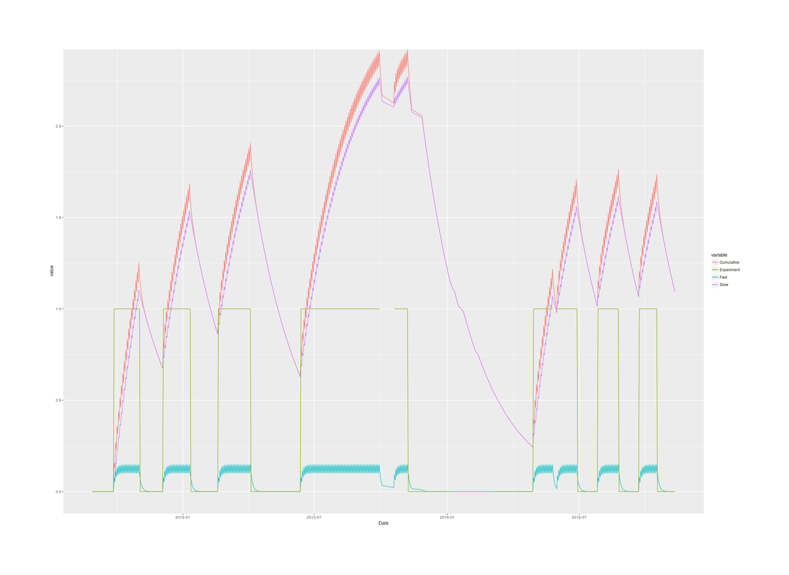
The slow totals turns out to reach far larger levels than the fast totals, and the cumulative is dominated by the slow total, so it makes more sense to avoid lumping them together: they are different biologically in size and half-life, are different parts of the body (the fast seems to be circulating magnesium while the slow corresponds to muscle & skeleton, I think 1966 suggests), and if they act differently, using the total would hide that, and if they don’t, they’ll add up to the same thing anyway.
bo <- brm(MP ~ Date.int + Dose.cumulative.slow + I(Dose.cumulative.slow^2) + Dose.cumulative.fast +  I(Dose.cumulative.fast^2), prior=c(prior(normal(0,0.005), "b")), autocor=cor_arma(~1, p=0, q=1), control = list(adapt_delta = 0.95, max_treedepth=15), iter=30000, chains=29, cores=29, data=magnesium); bo;
# Samples: 29 chains, each with iter = 30000; warmup = 15000; thin = 1;
#          total post-warmup samples = 435000
#
# Correlation Structures:
#       Estimate Est.Error l-95% CI u-95% CI Eff.Sample Rhat
# ma[1]     0.14      0.04     0.07     0.22      39314 1.00
#
# Population-Level Effects:
#                         Estimate Est.Error l-95% CI u-95% CI Eff.Sample Rhat
# Intercept                   9.01      1.88     5.33    12.70     435000 1.00
# Date.int                   -0.00      0.00    -0.00    -0.00     435000 1.00
# Dose.cumulative.slow        0.00      0.00    -0.00     0.00     435000 1.00
# IDose.cumulative.slowE2    -0.00      0.00    -0.00     0.00     435000 1.00
# Dose.cumulative.fast        0.00      0.00    -0.01     0.01      34194 1.00
# IDose.cumulative.fastE2    -0.00      0.00    -0.00     0.00      47501 1.00
#
# Family Specific Parameters:
#       Estimate Est.Error l-95% CI u-95% CI Eff.Sample Rhat
# sigma     0.63      0.02     0.60     0.66      45975 1.00
fixef(bo); waic(b,bo)
#                                Estimate      Est.Error            Q2.5           Q97.5
# Intercept                9.01339178e+00 1.88242899e+00  5.32696382e+00  1.27043508e+01
# Date.int                -3.52343153e-04 1.13874214e-04 -5.75665506e-04 -1.29252046e-04
# Dose.cumulative.slow     2.37189034e-04 1.99625166e-04 -1.53223784e-04  6.29052489e-04
# IDose.cumulative.slowE2 -8.77790825e-08 9.71539135e-08 -2.78303424e-07  1.02399191e-07
# Dose.cumulative.fast     7.26503721e-04 4.54413745e-03 -8.18732787e-03  9.62905267e-03
# IDose.cumulative.fastE2 -3.74918432e-04 2.37853248e-04 -8.40790729e-04  9.08634153e-05
#           WAIC    SE
# b      1467.51 35.35
# bo     1468.41 35.45
# b - bo   -0.90  3.40
marginal_effects(bo, effects=c("Dose.cumulative.slow", "Dose.cumulative.fast"))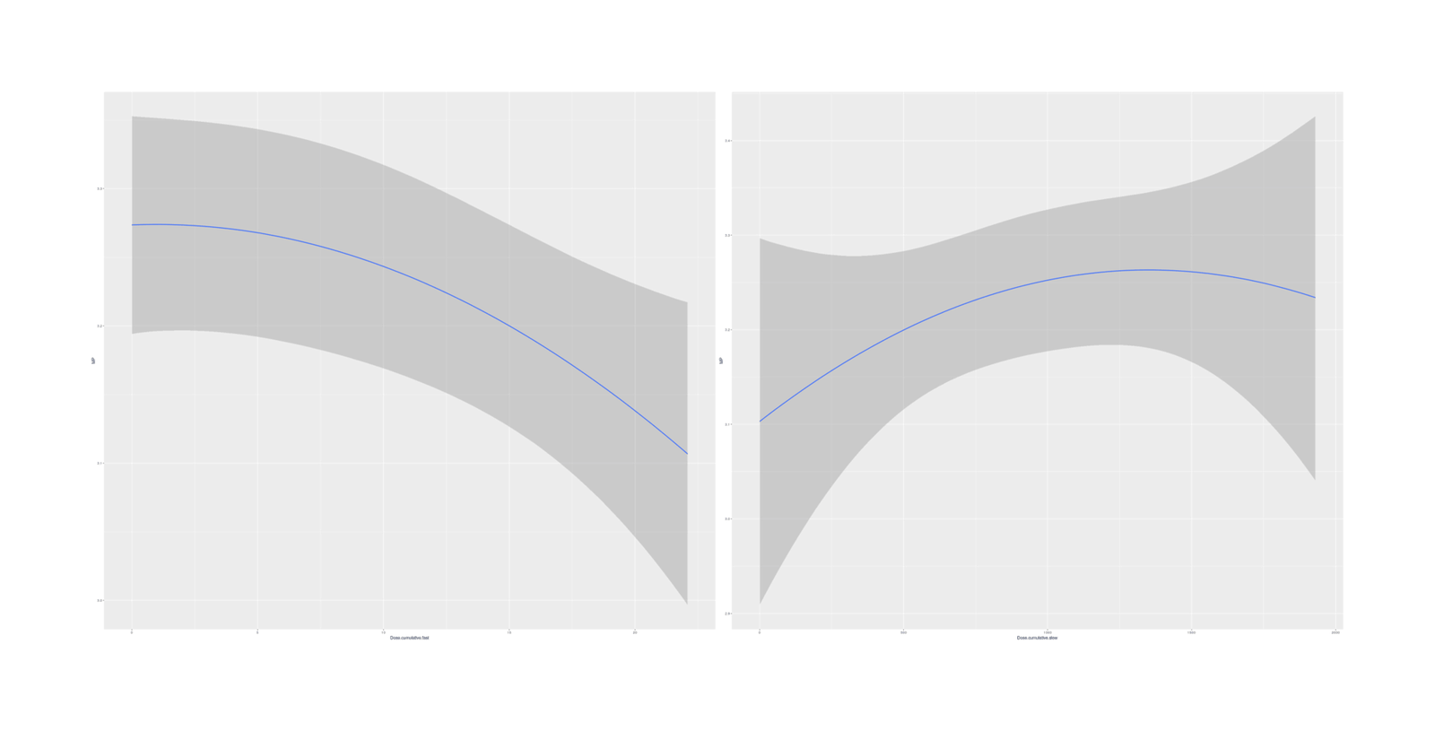
No especially strong quadratic dose-response curves emerge, and the model fit is just slightly worse than the simple linear total-dose model. It is interesting that the two quadratics hint at a short-term overload/harm but long-term benefit.
If we try fitting the quadratic with the Experimental indicator to see whether the effect of magnesium is captured by the two-dose model, the model is difficult to fit, requiring many more samples for convergence, but ultimately doesn’t
boe <- brm(MP ~ Date.int + Experimental + Dose.cumulative.slow + I(Dose.cumulative.slow^2) + Dose.cumulative.fast +
          I(Dose.cumulative.fast^2), prior=c(prior(normal(0,0.1/78)), prior(coef="Experimental", normal(0,0.1))),
          autocor=cor_arma(~1, p=0, q=1), iter=30000, chains=30, cores=30, control = list(adapt_delta = 0.99),
          data=magnesium)
summary(boe); fixef(boe); waic(b, bo, boe)
# Correlation Structures:
#       Estimate Est.Error l-95% CI u-95% CI Eff.Sample Rhat
# ma[1]     0.12      0.04     0.05     0.20      83841 1.00
#
# Population-Level Effects:
#                         Estimate Est.Error l-95% CI u-95% CI Eff.Sample Rhat
# Intercept                   8.71      1.83     5.11    12.30    1350000 1.00
# Date.int                   -0.00      0.00    -0.00    -0.00    1350000 1.00
# Experimental                0.02      0.07    -0.11     0.15      76746 1.00
# Dose.cumulative.slow        0.00      0.00    -0.00     0.00     491004 1.00
# IDose.cumulative.slowE2    -0.00      0.00    -0.00     0.00     542324 1.00
# Dose.cumulative.fast       -0.00      0.00    -0.00     0.00     115784 1.00
# IDose.cumulative.fastE2    -0.00      0.00    -0.00     0.00     138896 1.00
#
# Family Specific Parameters:
#       Estimate Est.Error l-95% CI u-95% CI Eff.Sample Rhat
# sigma     0.62      0.02     0.59     0.66      84156 1.00
#                                Estimate      Est.Error            Q2.5           Q97.5
# Intercept                8.71472231e+00 1.83496362e+00  5.11197732e+00  1.23036692e+01
# Date.int                -3.34069444e-04 1.11019111e-04 -5.51282372e-04 -1.15937711e-04
# Experimental             2.18818486e-02 6.51106318e-02 -1.05797456e-01  1.49466686e-01
# Dose.cumulative.slow     2.30301248e-04 1.88349858e-04 -1.39512183e-04  5.99674818e-04
# IDose.cumulative.slowE2 -9.66555633e-08 9.28998977e-08 -2.78618364e-07  8.55000738e-08
# Dose.cumulative.fast    -6.75864519e-06 6.65868030e-04 -1.31344906e-03  1.29675370e-03
# IDose.cumulative.fastE2 -3.49600899e-04 1.82533042e-04 -7.07912048e-04  7.38942643e-06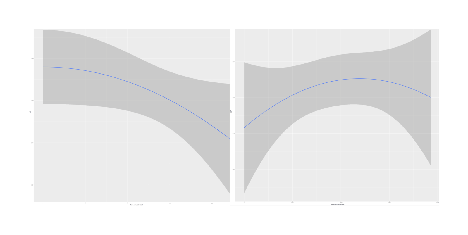
So it appears that the two-compartment model (at least, as I’ve implemented it, which may not be right) is not clearly superior; it may or may not be right, but the data is weak.
Additional Specifications
In desperation, I will proceed to torture the data with various ways to try to winkle out a temporal/accumulating effect.
One idea I had was to try different decay rates (of a single compartment, which would be perhaps the fast one), ranging from 1 day to 64 days, and use the horseshoe prior for variable selection to pick out the decay rate giving the most predictive moving-average. None of them popped out:
estimateDosing <- function(d) { magnesium$Dose %>% accumulate(function(cm, prv) { prv + (1-(0.5/d))*cm} ) }
magnesium$Dose.1d <- estimateDosing(1)
magnesium$Dose.2d <- estimateDosing(2)
magnesium$Dose.4d <- estimateDosing(4)
magnesium$Dose.8d <- estimateDosing(8)
magnesium$Dose.16d <- estimateDosing(16)
magnesium$Dose.32d <- estimateDosing(32)
magnesium$Dose.64d <- estimateDosing(64)

bod <- brm(MP ~ Date.int + Dose + Dose.1d + Dose.2d + Dose.4d + Dose.8d + Dose.16d + Dose.32d + Dose.64d,
    prior=c(set_prior("horseshoe(1, par_ratio=(1/7))")), iter=15000, chains=30, cores=30, data=magnesium)
summary(bod); fixef(bod)
# Population-Level Effects:
#           Estimate Est.Error l-95% CI u-95% CI Eff.Sample Rhat
# Intercept     6.38      2.24     2.65    10.73      11367 1.00
# Date.int     -0.00      0.00    -0.00     0.00      11203 1.00
# Dose         -0.00      0.00    -0.00     0.00      22772 1.00
# Dose.1d      -0.00      0.00    -0.00     0.00      16871 1.00
# Dose.2d      -0.00      0.00    -0.00     0.00       9947 1.00
# Dose.4d      -0.00      0.00    -0.00     0.00      13362 1.00
# Dose.8d      -0.00      0.00    -0.00     0.00       4789 1.01
# Dose.16d      0.00      0.00    -0.00     0.00       3778 1.01
# Dose.32d      0.00      0.00    -0.00     0.00       3681 1.01
# Dose.64d     -0.00      0.00    -0.00     0.00       4858 1.01
#
# Family Specific Parameters:
#       Estimate Est.Error l-95% CI u-95% CI Eff.Sample Rhat
# sigma     0.63      0.02     0.60     0.67      23631 1.00
# ...
#                  Estimate      Est.Error            Q2.5          Q97.5
# Intercept  6.37662456e+00 2.235888108006  2.649424916291 1.07293860e+01
# Date.int  -1.87427217e-04 0.000135929535 -0.000451826065 4.02780509e-05
# Dose      -9.83247484e-05 0.000398884863 -0.001201592100 5.62706619e-04
# Dose.1d   -1.14355053e-04 0.000490526386 -0.001424678384 6.96386862e-04
# Dose.2d   -1.23935090e-04 0.000432495370 -0.001206503256 5.95745260e-04
# Dose.4d   -1.84854122e-04 0.000372559311 -0.001123141480 3.49011680e-04
# Dose.8d   -1.63414873e-04 0.000337226934 -0.001082742030 2.72433040e-04
# Dose.16d   5.59172067e-05 0.000248260879 -0.000414186231 6.79183708e-04
# Dose.32d   1.55059360e-04 0.000227871520 -0.000104605208 7.47809143e-04
# Dose.64d  -7.71631435e-05 0.000106139588 -0.000342571572 5.31762310e-05
A similar method is lagging, just shifting the dose and estimating an attenuation, which didn’t work either:
magnesium$Lag.1 <- c(rep(0,1), magnesium$Dose)[1:nrow(magnesium)]
magnesium$Lag.2 <- c(rep(0,2), magnesium$Dose)[1:nrow(magnesium)]
magnesium$Lag.3 <- c(rep(0,3), magnesium$Dose)[1:nrow(magnesium)]
magnesium$Lag.4 <- c(rep(0,4), magnesium$Dose)[1:nrow(magnesium)]
magnesium$Lag.5 <- c(rep(0,5), magnesium$Dose)[1:nrow(magnesium)]
magnesium$Lag.6 <- c(rep(0,6), magnesium$Dose)[1:nrow(magnesium)]
magnesium$Lag.7 <- c(rep(0,7), magnesium$Dose)[1:nrow(magnesium)]
bol <- brm(MP ~ Date.int + Dose + Lag.1 + Lag.2 + Lag.3 + Lag.4 + Lag.5 + Lag.6 + Lag.7,
    prior=c(prior(normal(0,0.01))), iter=5000, chains=30, cores=30, data=magnesium)
summary(bol); fixef(bol)
# Population-Level Effects:
#           Estimate Est.Error l-95% CI u-95% CI Eff.Sample Rhat
# Intercept     8.34      1.62     5.16    11.52      75000 1.00
# Date.int     -0.00      0.00    -0.00    -0.00      75000 1.00
# Dose          0.00      0.00    -0.00     0.00      75000 1.00
# Lag.1         0.00      0.00    -0.00     0.00      75000 1.00
# Lag.2        -0.00      0.00    -0.01     0.00      60789 1.00
# Lag.3        -0.00      0.00    -0.01     0.00      62034 1.00
# Lag.4        -0.00      0.00    -0.01     0.00      62263 1.00
# Lag.5         0.00      0.00    -0.00     0.01      60792 1.00
# Lag.6         0.00      0.00    -0.00     0.00      75000 1.00
# Lag.7        -0.00      0.00    -0.00     0.00      75000 1.00
#
# Family Specific Parameters:
#       Estimate Est.Error l-95% CI u-95% CI Eff.Sample Rhat
# sigma     0.64      0.02     0.60     0.67      68165 1.00
#
# Samples were drawn using sampling(NUTS). For each parameter, Eff.Sample
# is a crude measure of effective sample size, and Rhat is the potential
# scale reduction factor on split chains (at convergence, Rhat = 1).
#                  Estimate      Est.Error            Q2.5          Q97.5
# Intercept  8.343749825167 1.62108462e+00  5.164844564711 11.52433155127
# Date.int  -0.000305389794 9.69037305e-05 -0.000495385229 -0.00011560533
# Dose       0.001125326534 1.89417227e-03 -0.002587631351  0.00483233217
# Lag.1      0.000259731777 1.88856710e-03 -0.003464743028  0.00398431704
# Lag.2     -0.002630603643 2.58733392e-03 -0.007694762066  0.00246824541
# Lag.3     -0.003248745460 2.58131724e-03 -0.008338464544  0.00179576211
# Lag.4     -0.000669146992 2.56489651e-03 -0.005715930399  0.00435186920
# Lag.5      0.002623359249 2.59021313e-03 -0.002451459184  0.00773690535
# Lag.6      0.000608268232 1.89271318e-03 -0.003081445775  0.00433930503
# Lag.7     -0.000160728821 1.89947146e-03 -0.003881042703  0.00358413020
brms does support formal ARIMA time-series models, so I considered similar ones which add ARIMA (to the response variable, MP) with lags up to 7 days and a moving-average, a 1-day lag+moving-average, and just a moving-average. (brms does not, as far as I can tell, support inference on the ARIMA parameters themselves other than in the generic sense of allowing you to fit multiple discrete models and then comparing with waic/loo etc.)
barma71 <- brm(MP ~ Dose, autocor=cor_arma(~1, p=7, q=1), iter=5000, chains=30, cores=30, data=magnesium); summary(barma71); fixef(barma71)
# Correlation Structures:
#       Estimate Est.Error l-95% CI u-95% CI Eff.Sample Rhat
# ar[1]     0.13      0.52    -0.79     0.94      13907 1.00
# ar[2]    -0.04      0.09    -0.20     0.12      15956 1.00
# ar[3]     0.02      0.05    -0.08     0.11      30385 1.00
# ar[4]    -0.03      0.04    -0.11     0.05      44092 1.00
# ar[5]     0.03      0.04    -0.05     0.12      35208 1.00
# ar[6]     0.00      0.05    -0.09     0.09      32015 1.00
# ar[7]     0.02      0.04    -0.05     0.10      50915 1.00
# ma[1]     0.01      0.52    -0.79     0.93      13888 1.00
#
# Population-Level Effects:
#           Estimate Est.Error l-95% CI u-95% CI Eff.Sample Rhat
# Intercept     8.22      1.93     4.42    12.01      74914 1.00
# Date.int     -0.00      0.00    -0.00    -0.00      74892 1.00
# Dose         -0.00      0.00    -0.00     0.00      75000 1.00
#
# Family Specific Parameters:
#       Estimate Est.Error l-95% CI u-95% CI Eff.Sample Rhat
# sigma     0.63      0.02     0.60     0.66      60937 1.00
#
# Samples were drawn using sampling(NUTS). For each parameter, Eff.Sample
# is a crude measure of effective sample size, and Rhat is the potential
# scale reduction factor on split chains (at convergence, Rhat = 1).
# Warning message:
# There were 17 divergent transitions after warmup. Increasing adapt_delta above 0.8 may help.
# See https://mc-stan.org/misc/warnings.html#divergent-transitions-after-warmup
#                  Estimate      Est.Error            Q2.5           Q97.5
# Intercept  8.222000498575 1.932432753905  4.416327738099  1.20085926e+01
# Date.int  -0.000299167802 0.000115613136 -0.000525771625 -7.13583711e-05
# Dose      -0.001149187774 0.000597896272 -0.002324613368  2.89226774e-05

barma11 <- brm(MP ~ Dose, autocor=cor_arma(~1, p=1, q=1), iter=5000, chains=30, cores=30, data=magnesium); summary(bama11); fixef(bama11)
# Correlation Structures:
#       Estimate Est.Error l-95% CI u-95% CI Eff.Sample Rhat
# ar[1]    -0.10      0.27    -0.62     0.44      28289 1.00
# ma[1]     0.25      0.27    -0.31     0.72      28510 1.00
#
# Population-Level Effects:
#           Estimate Est.Error l-95% CI u-95% CI Eff.Sample Rhat
# Intercept     3.22      0.03     3.17     3.28      47473 1.00
# Dose         -0.00      0.00    -0.00     0.00      75000 1.00
#
# Family Specific Parameters:
#       Estimate Est.Error l-95% CI u-95% CI Eff.Sample Rhat
# sigma     0.63      0.02     0.60     0.66      43505 1.00

bma <- brm(MP ~ Date.int + Dose, autocor=cor_arma(~1, p=0, q=1), iter=10000, chains=30, cores=30, data=magnesium); summary(bma); fixef(bma)
# Correlation Structures:
#       Estimate Est.Error l-95% CI u-95% CI Eff.Sample Rhat
# ma[1]     0.15      0.04     0.07     0.22      85325 1.00
#
# Population-Level Effects:
#           Estimate Est.Error l-95% CI u-95% CI Eff.Sample Rhat
# Intercept     8.25      1.84     4.65    11.83     150000 1.00
# Date.int     -0.00      0.00    -0.00    -0.00     150000 1.00
# Dose         -0.00      0.00    -0.00     0.00     150000 1.00
#
# Family Specific Parameters:
#       Estimate Est.Error l-95% CI u-95% CI Eff.Sample Rhat
# sigma     0.63      0.02     0.60     0.66      85214 1.00
#
# Samples were drawn using sampling(NUTS). For each parameter, Eff.Sample
# is a crude measure of effective sample size, and Rhat is the potential
# scale reduction factor on split chains (at convergence, Rhat = 1).
#                  Estimate      Est.Error            Q2.5           Q97.5
# Intercept  8.246820322945 1.836822995887  4.649351298371  1.18301614e+01
# Date.int  -0.000300629617 0.000109882242 -0.000515036715 -8.53722332e-05
# Dose      -0.001156989930 0.000636009833 -0.002405544347  8.80188844e-05
While I was at it, I threw some decision-tree methods, random forests & XGBoost, at it. Neither one performs much above chance, and both overfit:
library(randomForest)
r <- randomForest(MP ~ Date.int + Dose + Dose.1d + Dose.2d + Dose.4d + Dose.8d + Dose.16d + Dose.32d +
    Dose.64d + Lag.1 + Lag.2 + Lag.3 + Lag.4 + Lag.5 + Lag.6 + Lag.7, data=magnesium, importance=TRUE); r
#                Type of random forest: regression
#                      Number of trees: 500
# No. of variables tried at each split: 5
#
#           Mean of squared residuals: 0.45309365
#                     % Var explained: -11.5

library(xgboost)
xdf <- as.matrix(subset(magnesium, select=c("Date.int", "Dose", "Dose.1d", "Dose.2d",
    "Dose.4d", "Dose.8d", "Dose.16d", "Dose.32d", "Dose.64d", "Lag.1", "Lag.2", "Lag.3",
    "Lag.4", "Lag.5", "Lag.6", "Lag.7")))
xdt <- xgb.DMatrix(data=xdf, label=magnesium$MP)
xc <- xgb.cv(data=xdt, nrounds=20, nfold=5); xc
# ##### xgb.cv 5-folds
#  iter train_rmse_mean train_rmse_std test_rmse_mean test_rmse_std
#     1       1.9971932  0.00887113498      1.9965942 0.05663487645
#     2       1.4694444  0.00571063963      1.4738914 0.05622243389
#     3       1.1169894  0.00287774687      1.1322150 0.05330744639
#     4       0.8827894  0.00270631089      0.9221848 0.04989199156
#     5       0.7319208  0.00266308260      0.7998346 0.03957045891
#     6       0.6377054  0.00365968636      0.7273444 0.03119305256
#     7       0.5729780  0.00505585174      0.6925404 0.02332950090
#     8       0.5344652  0.00388501024      0.6750268 0.01660751560
#     9       0.5110230  0.00628505720      0.6688250 0.01083822294
#    10       0.4895788  0.00609432403      0.6633326 0.00994656782
#    11       0.4764658  0.00665422484      0.6616298 0.00788831770
#    12       0.4673910  0.00639055653      0.6622510 0.00830873304
#    13       0.4553722  0.00896999151      0.6623134 0.00798312374
#    14       0.4453348  0.01095618562      0.6634832 0.00916942418
#    15       0.4346564  0.01193689604      0.6643090 0.01121566110
#    16       0.4234282  0.01007038727      0.6668124 0.01150062806
#    17       0.4130764  0.01161052529      0.6686780 0.01166914274
#    18       0.4054248  0.01099076020      0.6720958 0.01327700370
#    19       0.3971520  0.01330724769      0.6726724 0.01219097106
#    20       0.3901480  0.01375990240      0.6741852 0.01182116611
External Links
-
Magnesium (first): 1
-
“The kidneys are crucial in magnesium homeostasis [18, 49–51] as serum magnesium concentration is primarily controlled by its excretion in urine [7]. Magnesium excretion follows a circadian rhythm, with maximal excretion occurring at night [15].” —Magnesium Basics↩︎