I compare my electric tea kettle to my stove kettle, and apply some simple statistical modeling verifying the electric is faster.
Electric kettles are faster, but I was curious how much faster my electric kettle heated water to high or boiling temperatures than does my stove-top kettle.
So I collected some data and compared them directly, trying out a number of statistical methods (principally: nonparametric & parametric tests of difference, linear & beta regression models, and a Bayesian measurement error model).
My electric kettle is faster than the stove-top kettle (the difference is both statistically-significant p≪0.01 & the posterior probability of difference is P ≈ 1), and the modeling suggests time to boil is largely predictable from a combination of volume, end-temperature, and kettle type.

My electric tea kettle is a “T-fal BF6138US Balanced Living 1-1750-Watt Electric Mini Kettle”, plugged into a normal electrical socket. The stove-top is a generic old metal kettle with a copper-clad bottom (it may have been intended to be a coffee percolator, given the shape, but it works well as a kettle) on a small resistance-heating coil stove burner (why not one of the 2 large coils? because the kettle bottom doesn’t cover the full surface area of the large burners); the stove is some very old small Gaffers-Sattler 4-burner stove/oven (no model name or number I could find in an accessible spot, but I’d guess it’s >30 years old).
Experiment
I began comparing them on the afternoon of 2015-02-16; the sea-level kitchen was at a warm 77.1℉ & 49% relative humidity (as measured by my Kongin temperature/humidity data logger). For measuring water volume, I used an ordinary 1-cup kitchen measuring cup (~235ml). And for measuring water temperature, I used a Taylor 9847N Antimicrobial Instant Read Digital Thermometer (Amazon), which claims to measure in units of .1℉ up to 450° and so can handle boiling water; I can’t seem to find accuracy numbers for this particular model, but I did find a listing saying that a similarly-priced model (the “Taylor 9877FDA Waterproof Pocket Digital Thermometer”) is accurate ±2°, which should be enough.
The relevant quantity of water for me is at least one of my fox tea mugs, which turns out to be almost exactly 2 cups of water ( or ~0.5l marking on electric kettle).
My testing procedure was as follows:
-
rinse out each kettle with fresh cold water from the tap (43°), fill with some, let sit for a few minutes
-
dump out all water from kettles
-
pour in with measuring cup 2-4 cups of cold water, put onto respective spots
-
adjust temperature setting on electric kettle if necessary
I divide the T-Fal temperature control into min/medium-low/medium/max.
-
start timer software, then turn on kettles as quickly as possible
(I’d guess this was a delay of ~3s; 3s has been subtracted from the times, but there’s still imprecision or measurement error in how fast I looked at the stopwatch or how long it took me to react or whether I jumped the gun.)
-
wait until electric kettle ‘clicks’, record time in seconds; turn electric kettle off, insert thermometer, and read final temperature of electrical kettle; then insert thermometer into stove-top kettle to measure stove-top kettle’s intermediate temperature
-
record time and 2 temperatures
-
place thermometer back into stove-top kettle, and watch the temperature reading until the stove-top’s temperature has reached the electric kettle’s final temperature; record the time
-
turn off stove heat, dump out hot water, return to step #1
This ensures that both kettles start equal, and the stove-top kettle is run only as long as it takes to reach the same temperature that the electric kettle reached; the intermediate temperature could also be useful for estimating temperature vs time curves.
I ran 12 tests at various combinations of water-volume and temperature setting.
I wound up not testing temperature settings thoroughly because once I began measuring final temperatures, I was dismayed to see that the T-fal temperature control was almost non-existent: 3/4s of the dial equated essentially to ‘boil’, and even the minimum heat setting still resulted in temperatures as high as 180°!—which makes the temperature control almost useless, since I think one needs colder water than that to prepare white teas and the more delicate greens… I am not happy with T-fal, but at least now I know what temperatures the dial settings correspond to.
To deal with the poor temperature control, I bought a cheap mechanical cooking thermometer, calibrated it, drilled a narrow hole through the plastic of the T-fal tea kettle, and inserted the probe down into the water area. Now I can see what the current water temperature is as it heats up, and shut it off early or dilute it with fresh water to get it to the target temperature. Perhaps not as convenient as a fully digital electric tea kettle, but it’s much cheaper and probably more reliable/durable; I may do this with future tea kettles as well.
Data
The data from each kettle (time in seconds, temperatures in Fahrenheit):
boiling <- read.csv(stdin(),header=TRUE)
Test,Setting,Type,Volume.cups,Time,Temp.final,Temp.intermediate.stove
1,max,electric,2,144,210,120
1,max,stove,2,344,210,120
2,max,electric,3,199,211,108
2,max,stove,3,665,211,108
3,max,electric,3,210,211,120
3,max,stove,3,701,211,120
4,max,electric,2,141,211,107
4,max,stove,2,524,211,107
5,medium,electric,2,142,209,130
5,medium,stove,2,399,209,130
6,medium-low,electric,2,145,207,131
6,medium-low,stove,2,408,207,131
7,min,electric,2,110,190,101
7,min,stove,2,423,190,101
8,min,electric,3,146,180,108
8,min,stove,3,435,180,108
9,min,electric,4,178,172,99
9,min,stove,4,567,172,99
10,min,electric,2,105,186,106
10,min,stove,2,362,186,106
11,min,electric,2,109,187,108
11,min,stove,2,331,187,108
12,min,electric,2,113,187,114
12,min,stove,2,341,187,114
Analysis
There many ways to analyze this data: are we interested in the mean difference in seconds over all combinations of volume/final-temperature, as a two-sample or paired-sample? In modeling the time it takes? In the ratio or relative speed of electric and stove-top? In correcting for the measurement error (±2° for each temperature measurement, and perhaps also how much water was in each)? We could look at all of them.
Hypothesis Testing
Means, ratios, and tests of difference:
abs(mean(boiling[boiling$Type=="electric",]$Time) - mean(boiling[boiling$Type=="stove",]$Time))
# [1] 313.1666667
boiling[boiling$Type=="electric",]$Time / boiling[boiling$Type=="stove",]$Time
#  [1] 0.4186046512 0.2992481203 0.2995720399 0.2690839695 0.3558897243 0.3553921569 0.2600472813
#  [8] 0.3356321839 0.3139329806 0.2900552486 0.3293051360 0.3313782991
summary(boiling[boiling$Type=="electric",]$Time / boiling[boiling$Type=="stove",]$Time)
#    Min.   1st Qu.    Median      Mean   3rd Qu.      Max.
# 0.2600473 0.2969499 0.3216191 0.3215118 0.3405722 0.4186047
wilcox.test(Time ~ Type, paired=TRUE, data=boiling)
#
#   Wilcoxon signed rank test with continuity correction
#
# data:  Time by Type
# V = 0, p-value = 0.002516
# alternative hypothesis: true location shift is not equal to 0
wilcox.test(Time ~ Type, paired=FALSE, data=boiling)
#
#   Wilcoxon rank sum test
#
# data:  Time by Type
# W = 0, p-value = 7.396e-07
# alternative hypothesis: true location shift is not equal to 0
t.test(Time ~ Type, data=boiling)
#
#   Welch Two Sample t-test
#
# data:  Time by Type
# t = -8.2263, df = 12.648, p-value = 1.983e-06
# alternative hypothesis: true difference in means is not equal to 0
# 95% confidence interval:
#  -395.6429254 -230.6904079
# sample estimates:
# mean in group electric    mean in group stove
#            145.1666667            458.3333333
t.test(Time ~ Type, paired=TRUE, data=boiling)
#
#     Paired t-test
#
# data:  Time by Type
# t = -11.1897, df = 11, p-value = 2.378e-07
# alternative hypothesis: true difference in means is not equal to 0
# 95% confidence interval:
#  -374.7655610 -251.5677723
# sample estimates:
# mean of the differences
#            -313.1666667
So the electric kettle is, as expected, faster—by 5 minutes on average, ranging from 4x faster to 2x faster, and the advantage is statistically-significant. (Nothing surprising so far.)
Linear Regression
How much variance do the listed variables capture?
summary(lm(Time ~ Test + Temp.final + as.ordered(Setting) + Type + Volume.cups, data=boiling))
# ...
# Residuals:
#       Min        1Q    Median        3Q       Max
# -89.37786 -28.86586  12.18942  29.12054  93.64656
#
# Coefficients:
#                           Estimate   Std. Error  t value   Pr(>|t|)
# (Intercept)           -2619.607015  1179.160067 -2.22159 0.04108708
# Test                      5.808909     9.295290  0.62493 0.54082745
# Temp.final               11.696298     5.422822  2.15687 0.04657229
# as.ordered(Setting).L   124.978494   109.450857  1.14187 0.27031014
# as.ordered(Setting).Q    88.043187    54.791923  1.60686 0.12763657
# as.ordered(Setting).C    24.081255    48.488960  0.49663 0.62620135
# Typestove               313.166667    24.560050 12.75106 8.4966e-10
# Volume.cups             157.883148    38.444409  4.10679 0.00082473
#
# Residual standard error: 60.15959 on 16 degrees of freedom
# Multiple R-squared:  0.9257358, Adjusted R-squared:  0.8932452
# F-statistic: 28.49242 on 7 and 16 DF,  p-value: 6.927389e-08
summary(step(lm(Time ~ Test + Temp.final + as.ordered(Setting) + Type + Volume.cups, data=boiling)))
# ...Residuals:
#         Min          1Q      Median          3Q         Max
# -115.480920  -41.874831   -3.183459   38.182981  125.963323
#
# Coefficients:
#                Estimate  Std. Error  t value   Pr(>|t|)
# (Intercept) -835.055578  206.880137 -4.03642 0.00064609
# Temp.final     3.607011    0.934039  3.86174 0.00097187
# Typestove    313.166667   24.083037 13.00362  3.247e-11
# Volume.cups  111.948746   20.132673  5.56055  1.922e-05
#
# Residual standard error: 58.99115 on 20 degrees of freedom
# Multiple R-squared:  0.9107407, Adjusted R-squared:  0.8973518
# F-statistic: 68.02206 on 3 and 20 DF,  p-value: 1.138609e-10
Because I controlled water volume and volume and final-temperature, the mean difference should be identical, and it is, 313s. The signs are also appropriate and coefficients sensible: each additional degree is +3.6s, a cup is +111s, and the setting variable drops out as useless (as it should since it should be redundant with the final-temperature measurement) as does the test number (suggesting no major change over time as a result of testing).
We can plot the electric and stove-top data separately as 3D plots with residuals to see if any big issues jump out:
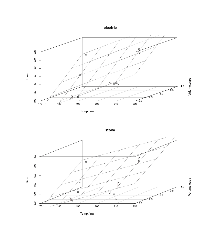
library(scatterplot3d)
plot3D <- function(k) {
    with(boiling[boiling$Type==k,], {
        b3d <- scatterplot3d(x=Temp.final, y=Volume.cups, Time, main=k);
        b3d$plane3d(my.lm <- lm(Time ~ Temp.final + Volume.cups), lty = "dotted");
        orig <- b3d$xyz.convert(Temp.final, Volume.cups, Time);
        plane <- b3d$xyz.convert(Temp.final, Volume.cups, fitted(my.lm));
        i.negpos <- 1 + (resid(my.lm) > 0);
        segments(orig$x, orig$y, plane$x, plane$y, col = c("blue", "red")[i.negpos], lty = (2:1)[i.negpos]);
        })
        }

png(file="~/wiki/doc/tea/gwern-tea-kettle-electricvstove.png", width = 680, height = 800)
    par(mfrow = c(2, 1))
    plot3D("electric")
    plot3D("stove")
invisible(dev.off())
It looks pretty good. But in general towards the edges the points seem systematically high or low, suggesting there might be a bit of nonlinearity, and the fit seems to be worse for the stove-top results, suggesting that’s noisier than electric (this could be due either to slight differences in setting the analogue temperature dial on the stove or perhaps differences in positioning on the burner coil).
Beta Regression
Regressing on the relative times / ratios, using the unusual beta regression, might be interesting; if electric was always 1:3, say, then one would expect the ratio to be constant and independent of the covariates, whereas if the ratio increases or decreases based on the covariates then that suggests some bending or flexing of the plane:
boilingW <- read.csv(stdin(),header=TRUE)
Test,Setting,Volume.cups,Time.electric,Time.stove,Time.ratio,Temp.final,Temp.intermediate.stove
1,max,2,144,344,0.4186046512,210,120
2,max,3,199,665,0.2992481203,211,108
3,max,3,210,701,0.2995720399,211,120
4,max,2,141,524,0.2690839695,211,107
5,medium,2,142,399,0.3558897243,209,130
6,medium-low,2,145,408,0.3553921569,207,131
7,min,2,110,423,0.2600472813,190,101
8,min,3,146,435,0.3356321839,180,108
9,min,4,178,567,0.3139329806,172,99
10,min,2,105,362,0.2900552486,186,106
11,min,2,109,331,0.329305136,187,108
12,min,2,113,341,0.3313782991,187,114

library(betareg)
summary(betareg(Time.ratio ~ Temp.final + as.ordered(Setting) + Volume.cups, data=boilingW))
# Standardized weighted residuals 2:
#        Min         1Q     Median         3Q        Max
# -3.0750244 -0.9096389  0.1394863  0.7292433  2.8146091
#
# Coefficients (mean model with logit link):
#                          Estimate  Std. Error  z value Pr(>|z|)
# (Intercept)            7.49624231  4.15031174  1.80619 0.070889
# Temp.final            -0.03782627  0.01921650 -1.96843 0.049019
# as.ordered(Setting).L -0.73487186  0.36540077 -2.01114 0.044311
# as.ordered(Setting).Q -0.47817927  0.19405990 -2.46408 0.013737
# as.ordered(Setting).C -0.18696030  0.16717555 -1.11835 0.263419
# Volume.cups           -0.22934320  0.13345514 -1.71850 0.085705
#
# Phi coefficients (precision model with identity link):
#        Estimate Std. Error z value Pr(>|z|)
# (phi) 201.71768   82.16848 2.45493 0.014091
#
# Type of estimator: ML (maximum likelihood)
# Log-likelihood: 24.01264 on 7 Df
# Pseudo R-squared: 0.3653261
# Number of iterations: 751 (BFGS) + 3 (Fisher scoring)
Excluding the Setting variable, it looks like the temperature and volume may affect the timing, but not much.
SEM
Moving on to measurement error, one favored way of handling measurement error is through latent variables and a structural equation model, which in this case we might model in lavaan this way:
library(lavaan)
Kettle.model <- '
                Temp.final.true =~ Temp.final
                Time.true =~ Time
                Volume.cups.true =~ Volume.cups
                Time.true ~ Test + Temp.final.true + as.ordered(Setting) + Type + Volume.cups.true
               '
Kettle.fit <- sem(model = Kettle.model, data = boiling)
summary(Kettle.fit)
# lavaan (0.5-16) converged normally after 120 iterations
#
#   Number of observations                            24
#
#   Estimator                                         ML
#   Minimum Function Test Statistic               65.575
#   Degrees of freedom                                 6
#   P-value (Chi-square)                           0.000
#
# Parameter estimates:
#
#   Information                                 Expected
#   Standard Errors                             Standard
#
#                    Estimate  Std.err  Z-value  P(>|z|)
# Latent variables:
#   Temp.final.true =~
#     Temp.final        1.000
#   Time.true =~
#     Time              1.000
#   Volume.cups.true =~
#     Volume.cups       1.000
#
# Regressions:
#   Time.true ~
#     Test              6.572    6.394    1.028    0.304
#     Temp.final.tr     5.237    0.547    9.568    0.000
#     Setting           0.385   16.210    0.024    0.981
#     Type            313.163   18.009   17.390    0.000
#     Volume.cps.tr   126.450   15.055    8.399    0.000
But the latent variable step turns out to be a waste of time (eg. Temp.final.true =~ Temp.final 1.000), presumably because I don’t have multiple measurements of the same data which might allow an estimate of an underlying factor/latent variable, and so it’s the same as the linear model, more or less.
Bayesian Models
What I need is some way of expressing my prior information, like my guess that the temperature numbers are ±2° or the times ±3s… in a Bayesian measurement error model. JAGS comes to mind. (Stan is currently too new and hard to install.)
library(rjags)
model1<-"
model {
    for (i in 1:n) {
        Time[i] ~ dnorm(Time.hat[i], tau)
        Time.hat[i] <- a + b1*Test[i] + b2*Temp.final[i] + b3*Setting[i] + b4*Type[i] + b5*Volume.cups[i]
    }

    # intercept
    a  ~ dnorm(0, .00001)

    # coefficients
    b1 ~ dnorm(0, .00001)
    b2 ~ dnorm(0, .00001)
    b3 ~ dnorm(0, .00001)
    b4 ~ dnorm(0, .00001)
    b5 ~ dnorm(0, .00001)

    # convert SD to 'precision' unit that JAGS's distributions use instead
    sigma ~ dunif(0, 100)
    tau <- pow(sigma, -2)
}
"
j1 <- with(boiling, jags(data=list(n=nrow(boiling), Time=Time, Temp.final=Temp.final,
                                   Volume.cups=Volume.cups, Type=Type, Setting=Setting, Test=Test),
                         parameters.to.save=c("b1", "b2", "b3", "b4", "b5"),
                         model.file=textConnection(model1),
                         n.chains=getOption("mc.cores"), n.iter=100000))
j1
# Inference for Bugs model at "5", fit using jags,
#  4 chains, each with 1e+05 iterations (first 50000 discarded), n.thin = 50
#  n.sims = 4000 iterations saved
#          mu.vect sd.vect    2.5%     25%     50%     75%   97.5%  Rhat n.eff
# b1         2.156  10.191 -18.143  -4.569   2.085   9.022  22.003 1.001  4000
# b2        -0.406   1.266  -2.906  -1.265  -0.373   0.419   2.061 1.001  4000
# b3       -40.428  26.908 -96.024 -58.060 -40.351 -22.395  11.220 1.001  2700
# b4       308.501  28.348 253.075 289.747 308.563 327.221 363.598 1.001  4000
# b5        80.985  23.082  33.622  66.062  81.784  96.441 125.030 1.001  4000
# deviance 269.384   4.058 263.056 266.473 268.887 271.673 279.300 1.001  4000
#
# For each parameter, n.eff is a crude measure of effective sample size,
# and Rhat is the potential scale reduction factor (at convergence, Rhat=1).
#
# DIC info (using the rule, pD = var(deviance)/2)
# pD = 8.2 and DIC = 277.6
# DIC is an estimate of expected predictive error (lower deviance is better).

## Stepwise-reduced variables:
model2<-"
model {
    for (i in 1:n) {
        Time[i] ~ dnorm(Time.hat[i], tau)
        Time.hat[i] <- a + b2 * Temp.final[i] + b4 * Type[i] + b5 * Volume.cups[i]
    }

    a  ~ dnorm(0, .00001)

    b2 ~ dnorm(0, .00001)
    b4 ~ dnorm(0, .00001)
    b5 ~ dnorm(0, .00001)

    tau <- pow(sigma, -2)
    sigma ~ dunif(0, 100)
}
"
j2 <- with(boiling, jags(data=list(n=nrow(boiling),Time=Time, Temp.final=Temp.final,
                                   Type=Type, Volume.cups=Volume.cups),
                         parameters.to.save=c("b2", "b4", "b5"), model.file=textConnection(model2),
                         n.chains=getOption("mc.cores"), n.iter=100000))
j2
#          mu.vect sd.vect    2.5%     25%     50%     75%   97.5%  Rhat n.eff
# b2         1.830   0.941  -0.140   1.235   1.875   2.474   3.594 1.001  4000
# b4       302.778  27.696 246.532 285.082 303.193 321.338 355.959 1.001  4000
# b5        90.526  22.306  46.052  75.869  90.848 105.883 133.368 1.001  4000
# deviance 268.859   4.767 261.564 265.238 268.276 271.854 279.749 1.001  4000
# ...
# DIC info (using the rule, pD = var(deviance)/2)
# pD = 11.4 and DIC = 280.2
# DIC is an estimate of expected predictive error (lower deviance is better).
The point-estimates are similar but pulled towards zero, as expected of noninformative priors. With a Bayesian analysis, we can ask directly, “what is the probability that the difference stove-top vs electric (b4) is >0?” A plot of the posterior samples shows that no sample is ≤0, so the probability that electric and stove-top differs is ~100%, which is comforting to know.
Measurement-error for Temp.final; we need to define a latent variable (true.Temp.final) which has our usual noninformative prior, but then we define how precise our measurement is (tau.Temp.final) by taking our two-degree estimate, converting it into units of standard deviations of the Temp.final data (2/14.093631), and then converting to the ‘precision’ unit (exponentiation followed by division):
model3<-"
model {
    for (i in 1:n) {
        true.Temp.final[i] ~ dnorm(0, .00001)
        Temp.final[i] ~ dnorm(true.Temp.final[i], tau.Temp.final)

        Time[i] ~ dnorm(Time.hat[i], tau)
        Time.hat[i] <- a + b2 * Temp.final[i] + b4 * Type[i] + b5 * Volume.cups[i]
    }
    a  ~ dnorm(0, .00001)

    b2 ~ dnorm(0, .00001)
    b4 ~ dnorm(0, .00001)
    b5 ~ dnorm(0, .00001)

    sigma ~ dunif(0, 100)
    tau <- pow(sigma, -2)

    tau.Temp.final <- 1 / pow((2/14.093631), 2)
}
"
j3 <- with(boiling, jags(data=list(n=nrow(boiling), Time=Time, Temp.final=Temp.final,
                                   Type=Type, Volume.cups=Volume.cups),
                         parameters.to.save=c("b2", "b4", "b5"), model.file=textConnection(model3),
                         n.chains=getOption("mc.cores"), n.iter=100000))
j3
#          mu.vect sd.vect    2.5%     25%     50%     75%   97.5%  Rhat n.eff
# b2         1.843   0.936  -0.106   1.238   1.889   2.497   3.570 1.001  4000
# b4       303.132  27.966 248.699 285.056 302.651 321.256 359.027 1.001  2900
# b5        89.503  21.985  43.631  75.713  90.076 104.306 130.206 1.001  4000
# deviance 242.944   8.204 228.833 237.013 242.222 248.095 260.670 1.001  2500
# ...
# DIC info (using the rule, pD = var(deviance)/2)
# pD = 33.6 and DIC = 276.6
# DIC is an estimate of expected predictive error (lower deviance is better).
In this case, ±2° degrees is precise enough, and the Temp.final variable just one of 3 variables used, that it seems to not make a big difference.
Another variable is how much water was in kettle. While I tried to measure cups as evenly as possible and shake out each kettle after rinsing, I couldn’t say it was hugely exact. There could easily have been a 5% difference between the kettles (and the standard deviation of the cups is not that small, it’s 0.653). So we’ll add that as a measurement error too:
model4<-"
model {
    for (i in 1:n) {
        true.Temp.final[i] ~ dnorm(0, .00001)
        Temp.final[i] ~ dnorm(true.Temp.final[i], tau.Temp.final)

        true.Volume.cups[i] ~ dnorm(0, .00001)
        Volume.cups[i] ~ dnorm(true.Volume.cups[i], tau.Volume.cups)

        Time[i] ~ dnorm(Time.hat[i], tau)
        Time.hat[i] <- a + b2 * Temp.final[i] + b4 * Type[i] + b5 * Volume.cups[i]
    }

    a  ~ dnorm(0, .00001)

    b2 ~ dnorm(0, .00001)
    b4 ~ dnorm(0, .00001)
    b5 ~ dnorm(0, .00001)

    sigma ~ dunif(0, 100)
    tau <- pow(sigma, -2)

    tau.Temp.final  <- 1 / pow((2/14.093631),       2)

    tau.Volume.cups <- 1 / pow((0.05/0.6538625482), 2)
}
"
j4 <- with(boiling, jags(data=list(n=nrow(boiling), Time=Time, Temp.final=Temp.final,
                                   Type=Type, Volume.cups=Volume.cups),
                         parameters.to.save=c("b2", "b4", "b5"), model.file=textConnection(model4),
                         n.chains=getOption("mc.cores"), n.iter=600000))
j4
#          mu.vect sd.vect    2.5%     25%     50%     75%   97.5%  Rhat n.eff
# b2         1.832   0.962  -0.213   1.210   1.885   2.488   3.603 1.001  4000
# b4       302.310  27.773 245.668 284.605 302.509 320.646 355.748 1.001  4000
# b5        89.655  21.768  44.154  75.561  90.428 104.743 129.892 1.002  2100
# deviance 188.133  10.943 169.013 180.519 187.413 195.102 211.908 1.001  4000
# ...
# DIC info (using the rule, pD = var(deviance)/2)
# pD = 59.9 and DIC = 248.0
While the DIC seems to have improved, the estimates look mostly the same. In this case, it seems that the variables are precise enough (measurement-errors small enough) that adjusting for them doesn’t change the results too much