HP: Methods of Rationality review statistics
Statistically modeling reviews for ongoing story with R.
The unprecedented gap in Methods of Rationality updates prompts musing about whether readership is increasing enough & what statistics one would use; I write code to download FF.net reviews, clean it, parse it, load into R, summarize the data & depict it graphically, run linear regression on a subset & all reviews, note the poor fit, develop a quadratic fit instead, and use it to predict future review quantities.
Then, I run a similar analysis on a competing fanfiction to find out when they will have equal total review-counts. A try at logarithmic fits fails; fitting a linear model to the previous 100 days of MoR and the competitor works much better, and they predict a convergence in <5 years.
A survival analysis finds no major anomalies in reviewer lifetimes, but an apparent increase in mortality for reviewers who started reviewing with later chapters, consistent with (but far from proving) the original theory that the later chapters’ delays are having negative effects.
In a LW comment, I asked:
I noticed in Eliezer’s latest [2012-11-01] MoR update that he now has 18,000 words written [of chapter 86], and even when that “chapter” is finished, he still doesn’t plan to post anything, on top of a drought that has now lasted more than half a year. This doesn’t seem very optimal from the point of view of gaining readers.
But I was wondering how one would quantify that—how one would estimate how many readers Eliezer’s MoR strategy of very rare huge dumps is costing him. Maybe survivorship curves, where survivorship is defined as “posting a review on FF.net”? So if say during the weekly MoR updates, a reader who posted a review of chapter X posted a review anywhere in X to X+n, that counts as survival of that reader. One problem here is that new readers are constantly arriving… You can’t simply say “X readers did not return from chapter 25 to chapter 30, while X+N did not return from chapter 85 to 86, therefore frequent updates are better” since you would expect the latter to be bigger simply because more people are reading. And even if you had data on unfavoriting or unfollowing, the important part is the opportunity cost—how many readers would have subscribed with regular updates
If you had total page views, that’d be another thing; you could look at conversions: what percentage of page views resulted in conversions to subscribers for the regular update period versus the feast/fame periods. But I don’t think FF.net provides it and while HP:MoR.com (set up 2011-06-13 as an alternative to FF.net; note the MoR subreddit was founded 2011-11-30] has Google Analytics, I don’t have access. Maybe one could look at each chapter pair-wise, and seeing what fraction of reviewers return? The growth might average out since we’re doing so many comparisons… But the delay is now so extreme this would fail: we’d expect a huge growth in reviewers from chapter 85 to chapter 86, for example, simply because it’s been like 8 months now—here too the problem is that the growth in reviewers will be less than what it “should be”. But how do we figure out “should be”?
After some additional discussion with clone_of_saturn, I’ve rejected the idea of survivorship curves; we thought correlations between duration and total review count might work, but interpretation was not clear. So the best current idea is: gather duration between each chapter, the # of reviews posted within X days (where X is something like 2 or 3), plot the points, and then see whether a line fits it better or a logarithm/logistic curve—to see whether growth slowed as the updates were spaced further apart.
Getting the data is the problem. It’s easy to get total reviews for each chapter since FF.net provides them. I don’t know of any way to get total reviews after X days posted, though! A script or program could probably do it, but I’m not sure I want to bother with all this work (especially since I don’t know how to do Bayesian line or logistic-fitting) if it’s not of interest to anyone or Eliezer would simply ignore any results.
I decided to take a stab at it.
Data
FanFiction.Net does not provide published dates for each chapter, so we’ll be working off solely the posted reviews. FF.net reviews for MoR are provided on 2223 pages (as of 2017-06-18), numbering from 1. If we start with https://www.fanfiction.net/r/5782108/85/1/, we can download them with a script enumerating the URLs & using string interpolation. Eyeballing a textual dump of the HTML (courtesy of elinks), it’s easy to extract with grep the line with user, chapter number, and date with a HTML string embedded as a link with each review, leading to this script:
for i in {1..2223}
do elinks -dump-width 1000 -no-numbering -no-references -dump https://www.fanfiction.net/r/5782108/0/$i/ \
     | grep "report review for abuse " | tee reviews.txt
done
Since page #1 is for the most recent URLs and we started with 1, the reviews were dumped newest to oldest: eg.
...
[IMG] report review for abuse SparklesandSunshine chapter 25 . 19h
[IMG] report review for abuse SparklesandSunshine chapter 24 . 19h
report review for abuse Emily chapter 7 . 6/12
[IMG] report review for abuse Ambassador666 chapter 17 . 6/12
[IMG] report review for abuse Teeners87 chapter 122 . 6/11
[IMG] report review for abuse Ryoji Mochizuki chapter 122 . 6/10
...
[IMG] report review for abuse Agent blue rose chapter 2 . 12/20/2016
report review for abuse Kuba Ober chapter 2 . 12/20/2016
[IMG] report review for abuse datnebnnii23 chapter 122 . 12/20/2016
report review for abuse Penguinjava chapter 101 . 12/20/2016
[IMG] report review for abuse Meerhawk chapter 122 . 12/20/2016
report review for abuse Laterreader12345 chapter 113 . 12/19/2016
...
We can clean this up with more shell scripting:
sed -e 's/\[IMG\] //' -e 's/.*for abuse //' -e 's/ \. chapter / /' reviews.txt >> filtered.txtThis gives us better looking data like:
Zethil1276 chapter 10 . 1h
Guest chapter 2 . 4h
SparklesandSunshine chapter 25 . 19h
SparklesandSunshine chapter 24 . 19h
Emily chapter 7 . 6/12
Ambassador666 chapter 17 . 6/12
Teeners87 chapter 122 . 6/11
Ryoji Mochizuki chapter 122 . 6/10
The spaces in names means we can’t simply do a search-and-replace to turn spaces into commas and call that a CSV which can easily be read in R; so more scripting, in Haskell this time (though I’m sure awk or something could do the job, I don’t know it):
import Data.List (intercalate)

main :: IO ()
main = do f <- readFile "filtered.txt"
          let parsed = map words (lines f)
          let unparsed = "User,Date,Chapter\n" ++ unlines (map unsplit parsed)
          writeFile "reviews.csv" unparsed

-- eg. "Ryoji Mochizuki chapter 122 . 6/10" → ["Ryoji", "Mochizuki", "6/10", "122"] → "Ryoji Mochizuki,6/10,22"
unsplit :: [String] -> String
unsplit xs = let chapter = last $ init $ init xs
                 date = last xs
                 user = intercalate " " $ takeWhile (/="chapter") xs
             in intercalate "," [user, date, chapter]
FF.net as of 2017 has changed its date format to vary by page, so the most recent reviews need to be hand-edited.
R
A runghc mor.hs later and our CSV of 33,332 reviews is ready for analysis in the R interpreter:
data <- read.csv("https://gwern.net/doc/lesswrong-survey/hpmor/2017-hpmor-reviews.csv")
data
# ...               User      Date Chapter
# 1          Zethil1276 6/18/2017      10
# 2               Guest 6/18/2017       2
# 3 SparklesandSunshine 6/18/2017      25
# 4 SparklesandSunshine 6/18/2017      24
# 5               Emily 6/12/2017       7
# 6       Ambassador666 6/12/2017      17
## Parse the date strings into R date objects
data$Date <- as.Date(data$Date,"%m/%d/%Y")
## Reorganize columns (we care more about the chapter & date reviews were given on
## than which user did a review):
data <- data.frame(Chapter=data$Chapter, Date=data$Date, User=data$User)
data <- data[order(data$Date),]
Descriptive
summary(data)
#     Chapter               Date                           User
#  Min.   : 1.00000   Min.   :2010-02-28   Guest            : 1798
#  1st Qu.: 10.00000   1st Qu.:2010-10-25   Anon             : 128
#  Median : 39.00000   Median :2012-03-26   anon             : 121
#  Mean   : 47.65211   Mean   :2012-09-20   The Anguished One: 121
#  3rd Qu.: 80.00000   3rd Qu.:2014-12-06   Montara          : 119
#  Max.   :122.00000   Max.   :2017-06-18   (Other)          :31044
#                                           NA's             :   1
The dates clearly indicate the slowdown in MoR posting, with the median chapter being posted all the way back in 201016ya. What does the per-day review pattern look like?
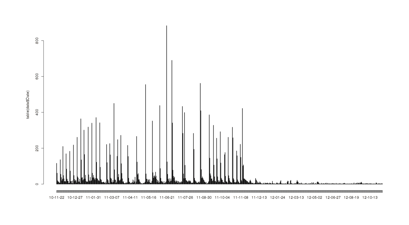
plot(table(data$Date))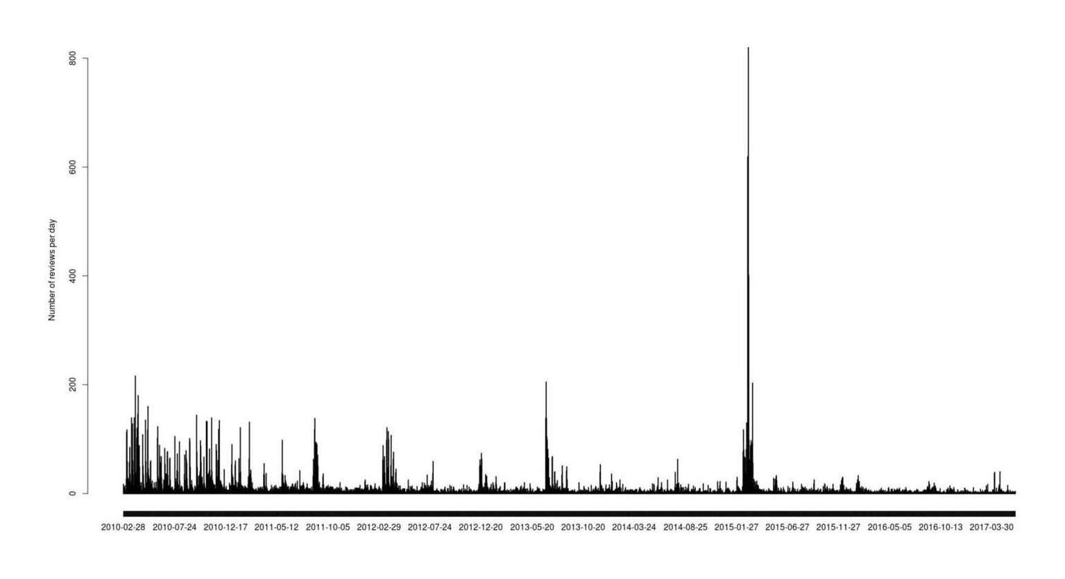
Reviews posted, by day
Quite spiky. At a guess, the days with huge spikes are new chapters with the final spike corresponding to the ending, while a low-level average of what looks like ~10 reviews a day holds steady over time. What’s the cumulative total of all reviews over time?
plot(unique(data$Date), cumsum(table(data$Date)), xlab="Date", ylab="Cumulative sum of FF.net reviews left on MoR over time")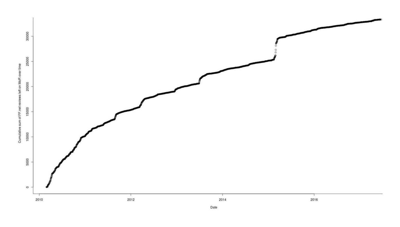
All (total cumulative) reviews posted, by day
When we plot each review by the chapter it was reviewing and the date it was posted, we see more clear patterns:
library(ggplot2)
qplot(data$Chapter, data$Date, color=as.ordered(data$Chapter)) +
    theme(legend.position = "none") + xlab("Chapter") + ylab("Date")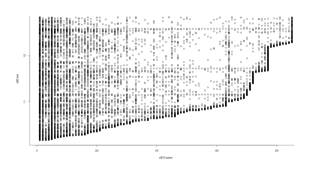
Scatterplot of all reviews, date posted versus chapter
Obviously no one can review a chapter before it was posted, which is the thick black line along the bottom. We can also see how the delays between chapters: originally very small, the gaps increase tremendously in the 70s chapters—just a few of the delays look like they cover the majority of the entire publishing lifespan of MoR! Other interesting observations is that chapter 1 and chapter 5 are extremely popular for reviewers, with hardly a day passing without review even as vast wastelands open up in 201214ya in chapters 40–60. A final curious observation is the presence of distinct horizontal lines; I am guessing that these are people prone to reviewing who are binging their way through MoR, leaving reviews on increasing chapters over short time periods.
Filtered Reviews
The next question is: if we plot only the subset of reviews which were made within 7 days of the first review, what does that look like?
## what's the total by each chapter?
totalReviews <- aggregate(Date ~ Chapter, length, data=data)
totalReviews$Date
#   [1] 1490 766 387 549 1896 815 650 563 550 758 568 325 401 409 333 412 547 420 401 420 321 273 290 346 196 325
#  [27]  362 193 180 227 186 230 211 156   63 123 131   83 211 133 151 242   86   58 223 281 405 147 180 128 237   99
#  [53]   72 206   62 166   96 231   96 154 154 196 342 263 166   58 171 151 301 341 242 421 153 308 227 266 574 209
#  [79]  189 328 274 135   90 185 301 175 280   50 426 169   53 119 134 119 169 123 107 192   74   79 178 153   83 181
# [105]   81   51 101 111   80   95   86 117 2080   88 204 104   96   60 144   77   84 544

earlyReviews <- integer(122)
for (i in 1:122) {
    reviews <- data[data$Chapter==i,]$Date
    published <- min(reviews)
    earlyReviews[i] <- sum(reviews < (published+7))
}
earlyReviews
#   [1]   17   11   13   34 326 190 203 209 296 281 117 136 162 144 126 153 195 198 159 201 127 124 140 110   92 141
#  [27]  192   96   91   43 113 169   76   88    5   34   73   17   48   71   88 128   17   10   40 163 238 100 121   81 148   50
#  [53]   31 164   32 127   62 164   66 116 107 139 151   54 104   19 106 104 170 185 104 172 124 211 163 181 113 168
#  [79]  136 299 206 104   69 139 102 109 120   32 350 144   27 103 104   84 136   89   78 101   21   36   56   54   56 149
# [105]   70   42   87   88   66   80   66 109 2026   67 191   94   89   50 128   65   67 233
How did chapter 5 get 326 reviews within 7 days when the previous ones were getting 10–30, you ask—might my data not be wrong? But if you check the chapter 5 reviews and scroll all the way down, you’ll find that people back in 201016ya were very chuffed by the Draco scenes.
Analysis
Linear Modeling
Moving onward, we want to graph the date and then fit a linear model (a line which minimizes the deviation of all of the points from it; I drew on a handout for R programming):
## turn vector into a plottable table & plot it
filtered <- data.frame(Chapter=c(1:122), Reviews=earlyReviews)
plot(filtered$Chapter, filtered$Reviews, xlab="Chapter",
    ylab="Reviews left on each chapter within 7 days of publication")

## run a linear model: is there any clear trend?
l <- lm(Reviews ~ Chapter, data=filtered); summary(l)
# ...Coefficients:
#                     Estimate Std. Error t value Pr(>|t|)
# (Intercept)      109.3701395 33.9635875 3.22022 0.0016484
# filtered$Chapter   0.3359780   0.4792406 0.70106 0.4846207
#
# Residual standard error: 186.4181 on 120° of freedom
# Multiple R-squared: 0.004079042, Adjusted R-squared: −0.0042203
# F-statistic: 0.4914898 on 1 and 120 DF,  p-value: 0.4846207

## the slope doesn't look very interesting...
## let's plot the regression line too:
abline(l)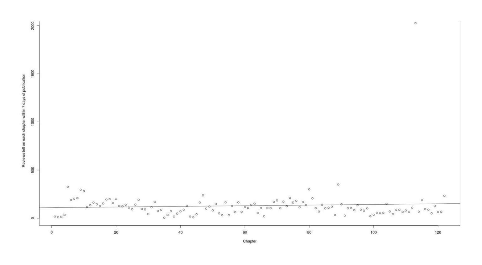
Graph reviews posted within a week, per chapter.
Look at the noise. We have some huge spikes in the early chapters, some sort of dip in the 40s-70s, and then a similar spread of highly and lowly reviewed chapters at the end. The linear model is basically just the average.
The readership of MoR did increase substantially over its run, so why is there such a small increase over time in the number of fans? Possibly most of the activity was drained over to Reddit as the subreddit started up in November 201115ya, and Ff.net reviews also decreased when the official website started up in June 201115ya. But those could only affect chapter 73 and later.
All Reviews
Same thing if we look at total reviews for each chapter:
filtered2 <- data.frame(Chapter=c(1:122), Reviews=totalReviews$Date)
plot(filtered2$Chapter, filtered2$Reviews, xlab="Chapter", ylab="Total reviews left on each chapter")
model2 <- lm(Reviews ~ Chapter, data=filtered2)
summary(model2)
# ...Coefficients:
#                Estimate Std. Error t value   Pr(>|t|)
# (Intercept) 460.8210270 50.7937240 9.07240 2.7651e-15
# Chapter      −3.0505352   0.7167209 −4.25624 4.1477e-05
#
# Residual standard error: 278.7948 on 120° of freedom
# Multiple R-squared: 0.1311624,   Adjusted R-squared: 0.1239221
# F-statistic: 18.11557 on 1 and 120 DF,  p-value: 4.147744e-05
abline(model2)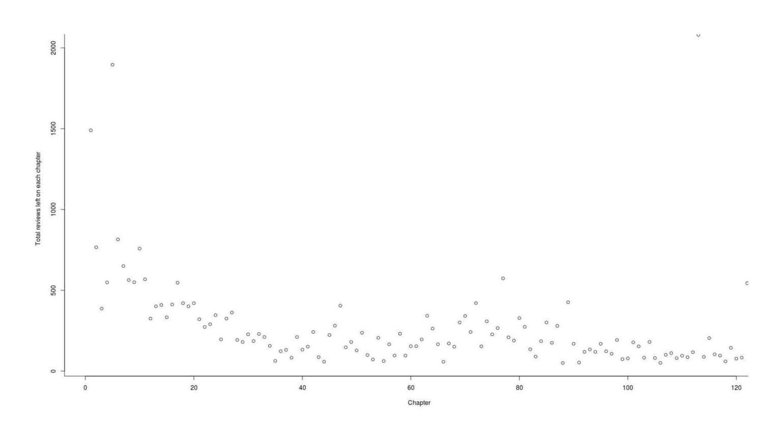
Graph all reviews by posted time and chapter
Fitting Quadratics
Looking at the line, the fit seems poor over all (large residuals) quite poor at the beginning and end—doesn’t it look like a big U? That sounds like a quadratic, so more Googling for R code and an hour or two later, I fit some quadratics to the 7-day reviews and the total reviews:
plot(filtered$Chapter, filtered$Reviews)
model <- lm(filtered$Reviews ~ filtered$Chapter + I(filtered$Chapter^2))
summary(model)
# ...Residuals:
#      Min       1Q   Median       3Q      Max
# −160.478 −42.795   −3.364   40.813 179.321
#
# Coefficients:
#                        Estimate Std. Error t value Pr(>|t|)
# (Intercept)           178.41168   22.70879   7.857 1.34e-11 ✱✱✱
# filtered$Chapter       −3.54725    1.21875 −2.911 0.00464 ✱✱
# I(filtered$Chapter^2)   0.04012    0.01373   2.922 0.00449 ✱✱
# ---
# Signif. codes: 0 ‘✱✱✱’ 0.001 ‘✱✱’ 0.01 ‘*’ 0.05 ‘.’ 0.1
#
# Residual standard error: 68.15 on 82° of freedom
# Multiple R-squared: 0.09533,    Adjusted R-squared: 0.07327
# F-statistic: 4.32 on 2 and 82 DF,  p-value: 0.01645

xx <- seq(min(filtered$Chapter),max(filtered$Chapter),len=200)
yy <- model$coef %*% rbind(1,xx,xx^2)
lines(xx,yy,lwd=2,col=3)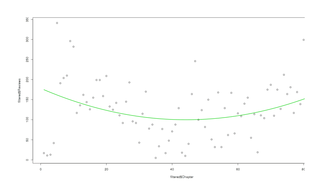
Fit a quadratic (U-curve) to the filtered review-count for each chapter
The quadratic fits nicely. And for total reviews, we observe a similar curve:
plot(filtered2$Chapter, filtered2$Reviews)
model2 <- lm(filtered2$Reviews ~ filtered2$Chapter + I(filtered2$Chapter^2))
# summary(model2)
# ...
# Residuals:
#     Min      1Q Median      3Q     Max
# −289.68 −56.83 −17.59   36.67 695.45
#
# Coefficients:
#                         Estimate Std. Error t value Pr(>|t|)
# (Intercept)            543.84019   41.43142 13.126 < 2e-16 ✱✱✱
# filtered2$Chapter      −16.88265    2.22356 −7.593 4.45e-11 ✱✱✱
# I(filtered2$Chapter^2)   0.16479    0.02505   6.578 4.17e-09 ✱✱✱
# ---
# Signif. codes: 0 ‘✱✱✱’ 0.001 ‘✱✱’ 0.01 ‘*’ 0.05 ‘.’ 0.1
#
# Residual standard error: 124.3 on 82° of freedom
# Multiple R-squared: 0.4518, Adjusted R-squared: 0.4384
# F-statistic: 33.79 on 2 and 82 DF,  p-value: 1.977e-11

xx <- seq(min(filtered2$Chapter),max(filtered2$Chapter),len=200)
yy <- model2$coef %*% rbind(1,xx,xx^2)
lines(xx,yy,lwd=2,col=3)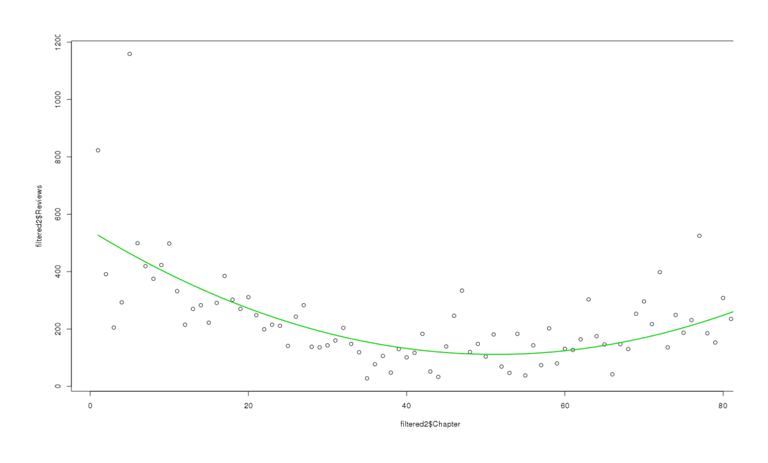
Fit a quadratic (U-curve) to the final 2012-11-03 review-count for each chapter
Predictions / Confidence Intervals
Linear models, even as a quadratic, are pretty simple. They don’t have to be a black box, and they’re interpretable the moment you are given the coefficients: ‘this’ times ‘that’ equals ‘that other thing’. We learned these things in middle school by hand-graphing functions. So it’s not hard to figure out what function our fitted lines represent, or to extend them rightwards to uncharted waters.
Our very first linear model for filtered$Reviews ~ filtered$Chapter told us that the coefficients were Intercept: 128.3773, filtered$Chapter: −0.0966. Going back to middle school math, the intercept is the y-intercept, the value of y when x = 0; then the other number must be how much we multiply x by.
So the linear model is simply this: y = −0.0966x + 128.3773. To make predictions, we substitute in for x as we please; so chapter 1 is −0.0966 × 1 + 128.3773 = 128.28, chapter 85 is −0.0966 × 85 + 128.3773 = 120.16 (well, what did you expect of a nearly-flat line?) and so on.
We can do this for the quadratic too; your ordinary quadratic looked like y = x2 + x + 1, so it’s easy to guess what the filled-in equivalent will be. We’ll look at total reviews this time (filtered2$Reviews ~ filtered2$Chapter + I(filtered2$Chapter^2)). The intercept was 543.84019, the first coefficient was −16.88265, and the third mystery number was 0.16479, so the new equation is y = 0.16479x2 + −16.88265x + 543.84019. What’s the prediction for chapter 86? 0.16479 × 862 + (−16.88265) × 86 + 543.8401 = 310.719. And for chapter 100, it’d go 0.16479 × (1002) + (−16.88265) × 100 + 543.8401 = 503.475.
Can we automate this? Yes. Continuing with total reviews per chapter:
x = filtered2$Chapter; y = filtered2$Reviews
model2 <- lm(y ~ x + I(x^2))
predict.lm(model2, newdata = data.frame(x = c(86:100)))
#        1        2        3        4        5        6        7        8
# 310.7242 322.3504 334.3061 346.5914 359.2063 372.1507 385.4248 399.0284
#        9       10       11       12       13       14       15
# 412.9616 427.2244 441.8168 456.7387 471.9903 487.5714 503.4821
(Notice that this use of predict spits out the same answers we calculated for chapter 86 and chapter 100.)
So for example, the fitted quadratic model predicts ~503 total reviews for chapter 100. Making further assumptions (the error in estimating is independent of time, normally distributed, has zero mean, and constant variance), we predict that our 95% confidence interval 215–792 total reviews of chapter 100:
predict.lm(model2, newdata = data.frame(x = 100), interval="prediction")
#        fit    lwr      upr
#   503.4821 215.05 791.9141
Clearly the model isn’t making very strong predictions because the standard error is so high. We get a similar result asking just for the 7-day reviews:
filtered=data.frame(Chapter=c(1:85),Reviews=earlyreviews)
y=filtered$Reviews; x=filtered$Chapter

model = lm(y ~ x + I(x^2))
model
# ...Coefficients:
# (Intercept)            x       I(x^2)
#   178.41168     −3.54725      0.04012
#
# predict.lm(model, newdata = data.frame(x = 100), interval="prediction")
#       fit      lwr      upr
# 1 224.925 66.83383 383.0162
This seems like a fairly reasonable prediction: 66–383 reviews posted within 7 days. But this is based purely off the model, is it taking into account that even the quadratic model has some pretty large residuals? Let’s plot an entire confidence band:
filtered <- data.frame(Chapter=c(1:85),Reviews=earlyreviews)
y <- filtered$Reviews; x = filtered$Chapter
plot(x, xlab="Chapter",
     y, ylab="Reviews posted within week",
     main="7-Day Reviews per Chapter with Quadratic Fit and 95% Prediction Intervals")

model <- lm(y ~ x + I(x^2))
xx <- seq(min(x),max(x),len=200)
yy <- model$coef %*% rbind(1,xx,xx^2)
lines(xx,yy,lwd=2,col=3)

prd <- predict(model, newdata = data.frame(x = c(1:85)), interval="prediction", type="response")
lines(c(1:85),prd[,2],col="red",lty=2)
lines(c(1:85),prd[,3],col="red",lty=2)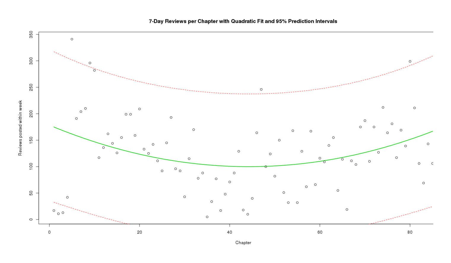
7-Day Reviews per Chapter with Quadratic Fit and 95% Prediction Intervals
The prediction bands look like they’re more or less living up to their claimed coverage (7⁄85 isn’t hugely far from 5⁄100) but do this by being very large and embarrassingly can’t even exclude zero. This should temper our forecasting enthusiasm. What might predict the residuals better? Day of week? Length of chapter update? Interval between updates? Hard to know.
Modeling Conclusions
Sadly, neither the quadratic nor the linear fits lend any support to the original notion that we could estimate how much readership MoR is being cost by the exponentially-slowing updates for the simple reason that the observed reviews per chapter do not match any simple increasing model of readership but a stranger U-curve (why do reviews decline so much in the middle when updates were quite regular?).
We could argue that the sluggishness of the recent upturn in the U-curve (in the 80s) is due to there only being a few humongous chapters, but those chapters are quantitatively and qualitatively different from the early chapters (especially chapter 5) so it’s not clear that any of them “should” have say, 341 reviews within a week.
Additional Graphs
Total cumulative MoR reviews as a function of time, with linear fit
Total MoR reviews vs time, quadratic fit
Total cumulative MoR reviews, 100 days prior to 2012-11-17, linear fit
The Review Race: Unexpected Circumstances Versus MoR
An interesting question is whether and when MoR will become the most-reviewed fanfiction on FFN (and by extension, one of the most-reviewed fanfictions of all time). It has already passed such hits as “Parachute” & “Fridays at Noon”, but the next competitor is Unexpected Circumstances (UC) at 24,163 reviews to MoR’s 18,9171.
Averaging
24.2k vs 19k is a large gap to cover. Some quick and dirty reasoning:
MoR: 18911 reviews, begun 02-28-10 or 992 days ago, so 18911/992 = 19.1 reviews per day (Status: in progress)
UC: 24163 reviews, begun 11-22-10 or 725 days ago, so 24,163/725 = 33.3 reviews per day (Status: complete)
Obviously if UC doesn’t see its average review rate decline, it’ll never be passed by MoR! But let’s assume the review rate has gone to zero (not too unrealistic a starting assumption, since UC is finished and MoR is not), how many days will it take MoR to catch up? (24163 - 18911) / (18911/992) = 275.5 or under a year.
Modeling
Descriptive Data and Graphs
We can take into account the existing review rates with the same techniques we used previously for investigating MoR review patterns. First, we can download & parse UC’s reviews the same way as before: make the obvious tweaks to the shell script, run the sed command, re-run the Haskell, then load into R & format:
for i in {1..1611};
do elinks -dump-width 1000 -no-numbering -no-references -dump https://www.fanfiction.net/r/6496709/0/$i/
    | grep "report review for abuse " >> reviews.txt;
done
sed -e 's/\[IMG\] //' -e 's/.*for abuse //' -e 's/ \. chapter / /' reviews.txt >> filtered.txt
runghc mor.hs
data <- read.table("https://gwern.net/doc/lesswrong-survey/hpmor/2012-uc-reviews.csv",header=TRUE, sep=",",quote="")
# Convert the date strings to R dates
data=data.frame(Chapter=data$Chapter, Date=as.Date(data$Date,"%m/%d/%Y"), User=data$User)
data
# Chapter Date User
# 1 39 12-11-14 REL57
# 2 27 12-11-13 Guest
# 3 26 12-11-13 Melanie
# 4 24 12-11-13 Melanie
# 5 39 12-11-13 Dream-with-your-heart
# 6 39 12-11-12 ebdarcy.qt4good
# 7 19 12-11-10 Guest
# 8 15 12-11-10 JD Thorn
# 9 39 12-11-09 shollyRK
# 10 9 12-11-08 of-Snowfall-and-Seagulls
# ...
summary(data)
# Chapter Date User
# Min. : 1.00 Min. :10-11-22 Guest : 54
# 1st Qu.:12.00 1st Qu.:11-02-26 AbruptlyChagrined : 39
# Median :22.00 Median :11-06-20 AlexaBrandonCullen: 39
# Mean :20.62 Mean :11-06-10 Angeldolphin01 : 39
# 3rd Qu.:29.00 3rd Qu.:11-09-09 AnjieNet : 39
# Max. :39.00 Max. :12-11-14 beachblonde2244 : 39
# (Other) :23915Unlike MoR, multiple people have reviewed all (39) chapters. Let’s look at total reviews posted each calendar day:
plot(table(data$Date))We’d like to see what a running or cumulative total reviews looks like: how fast is UC’s total review-count growing these days?
plot(cumsum(table(data$Date)))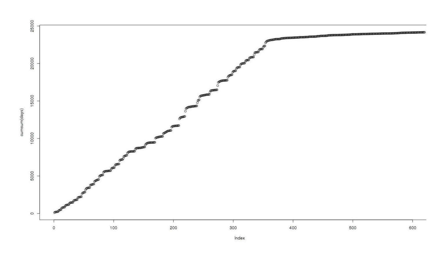
Total reviews as a function of time
Visually, it’s not quite a straight line, not quite a quadratic…
A graph of each day UC has existed against reviews left that day
We also get a similar graph to MoR if we graph by chapter instead, with thick bars indicating reviews left at the “latest” chapter while the series was updating, and many reviews left at the final chapter as people binge through UC:
plot(data$Chapter,data$Date)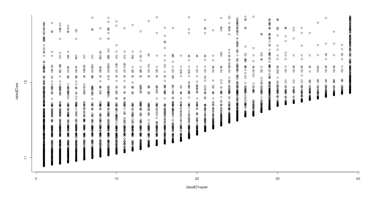
Total reviews on each chapter of UC
Let’s start modeling.
Linear Model
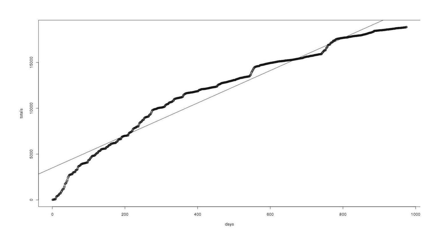
The linear doesn’t match well since it clearly is massively over-predicting future growth!
totals <- cumsum(table(data$Date))
days <- c(1:(length(totals)))
plot(days, totals)

model <- lm(totals ~ days)
abline(model)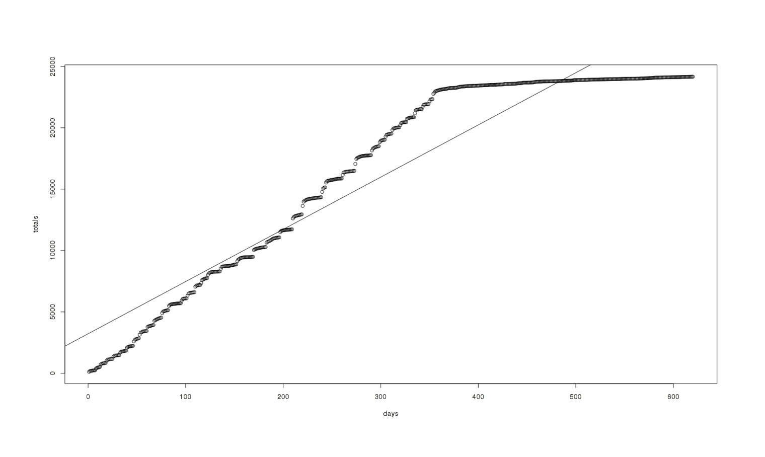
A graph of total reviews vs time with a (bad) linear fit overlaid
Quadratic Model
Well, the graph does look more like a quadratic, but this has another problem:
model <- lm(totals ~ days + I(days^2))
xx <- seq(min(days),max(days),len=200)
yy <- model$coef %*% rbind(1,xx,xx^2)
plot(days, totals)
lines(xx,yy,lwd=2,col=3)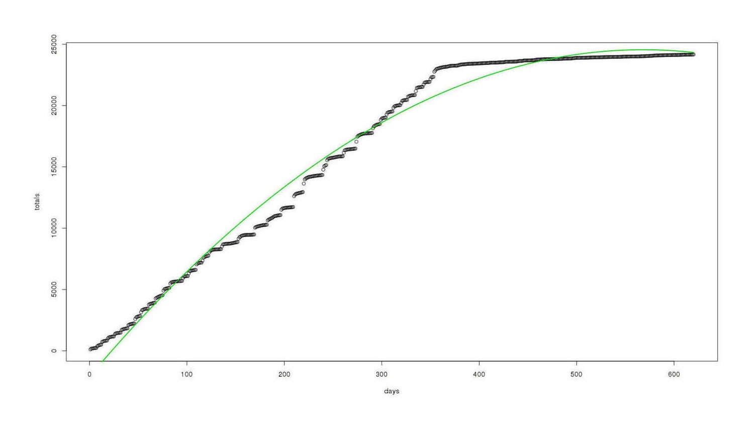
Same graph, better (but still bad) quadratic fit overlaid
It fits much better overall, but for our purposes it is still rubbish: it is now predicting negative growth in total review count (a parabola must come down, after all), which of course cannot happen since reviews are not deleted.
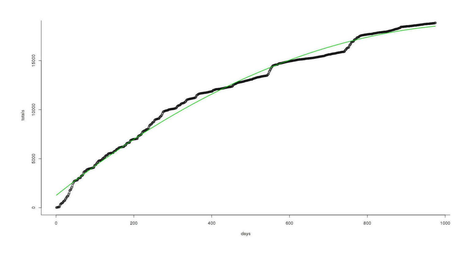
Logarithmic Model
We need a logarithmic function to try to model this “leveling-off” behavior:
logEstimate = lm(totals ~ log(days))
plot(days,predict(logEstimate),type='l',col='blue')
points(days,totals)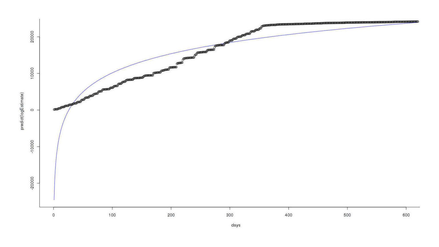
I’m a logarithm, and I’m OK…
The fit is very bad at the start, but the part we care about, recent reviews, seems better modeled than before. Progress! With a working model, let’s ask the original question: with these models predicting growth for UC and MoR, when do they finally have an equal number of reviews? We can use the predict.lm function to help us
## for MoR
predict.lm(logEstimate, newdata = data.frame(days = c(10000:20000)))
# ...
#     9993     9994     9995     9996     9997     9998     9999    10000
# 31781.54 31781.78 31782.03 31782.27 31782.52 31782.76 31783.01 31783.25
#    10001
# 31783.50

## for UC
predict.lm(logEstimate, newdata = data.frame(days = c(10000:20000)))
# ...
#     9993     9994     9995     9996     9997     9998     9999    10000
# 50129.51 50129.88 50130.26 50130.64 50131.02 50131.39 50131.77 50132.15
#    10001
# 50132.53
Growth in reviews has asymptoted for each way out at 10,000 days or 27 years, but still UC > MoR! This feels a little unlikely: the log function grows very slowly, but are the reviews really slowing down that much?
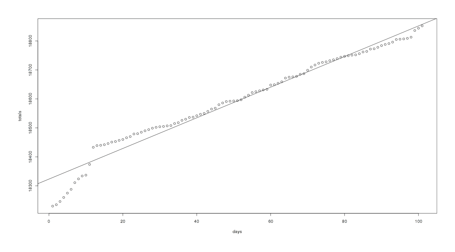
Linear Model Revisited
Let’s ask a more restricted question—instead of trying to model the entire set of reviews, why not look at just the most recent chunk, the one sans any updates (for both, sadly), say the last 100 days?
totals <- cumsum(table(data$Date))
totals <- totals[(length(totals)-100):length(totals)]
days <- c(1:(length(totals)))
days <- days[(length(days)-100):length(days)]
plot(days, totals)
model <- lm(totals ~ days)
summary(model)
# ...Residuals:
#      Min       1Q   Median       3Q      Max
# −18.4305 −4.4631   0.2601   7.4555 16.0125
#
# Coefficients:
#              Estimate Std. Error t value Pr(>|t|)
# (Intercept) 2.392e+04 1.769e+00 13517.26   <2e-16 ✱✱✱
# days        2.472e+00 3.012e-02    82.08   <2e-16 ✱✱✱
# ---
# Signif. codes: 0 ‘✱✱✱’ 0.001 ‘✱✱’ 0.01 ‘*’ 0.05 ‘.’ 0.1
#
# Residual standard error: 8.826 on 99° of freedom
# Multiple R-squared: 0.9855, Adjusted R-squared: 0.9854
# F-statistic: 6737 on 1 and 99 DF,  p-value: < 2.2e-16

abline(model)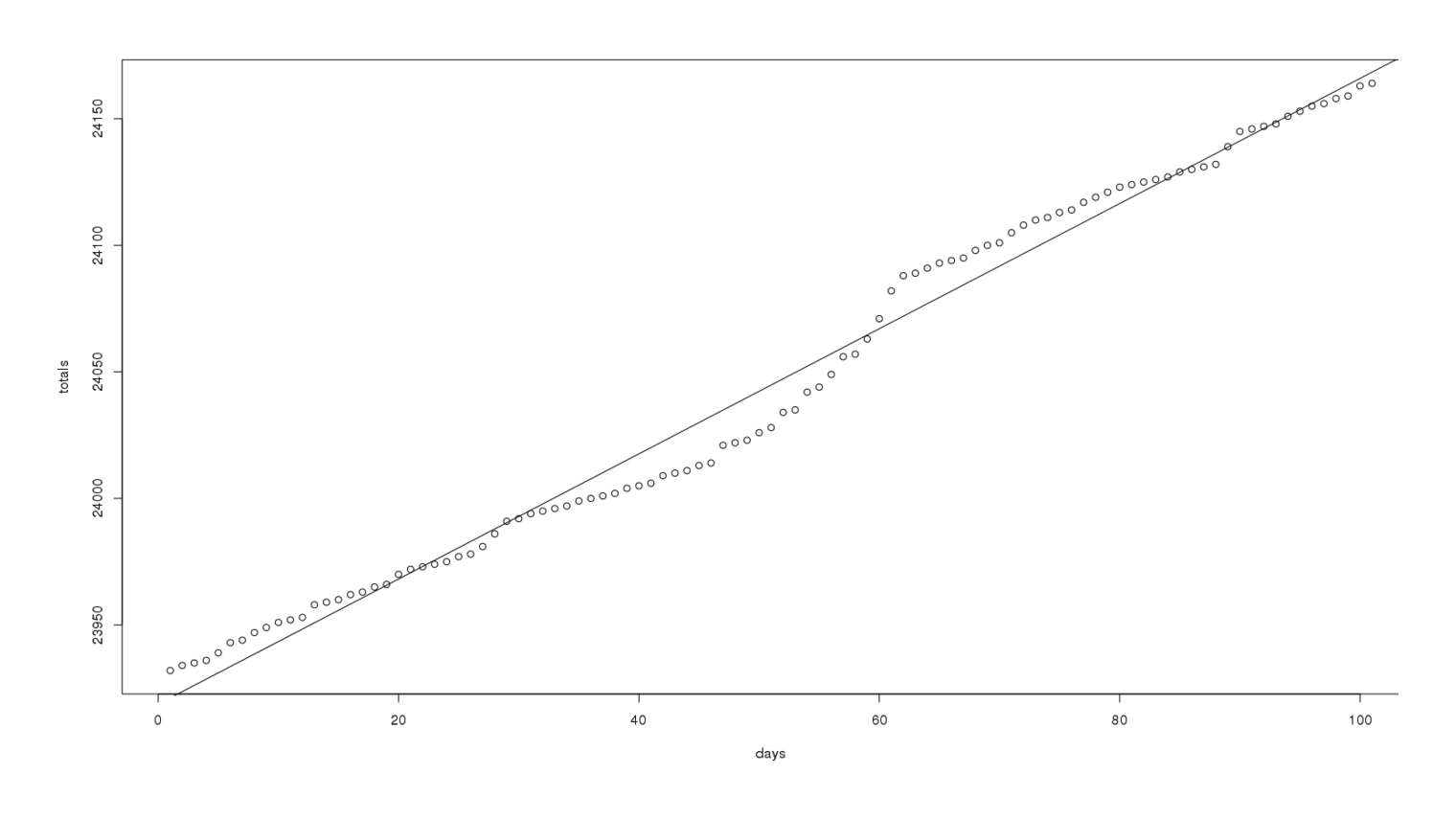
A linear fit to the last 100 days of UC reviews
That’s an impressive fit: visually a great match, relatively small residuals, extreme statistical-significance. (We saw a similar graph for MoR too.) So clearly the linear model is accurately describing recent reviews.
Predicting
Let’s use 2 models like that to make our predictions. We’ll extract the 2 coefficients which define a y = ax + c linear model, and solve for the equality:
## UC:
coefficients(model)
#  (Intercept)         days
# 23918.704158     2.472312

## MoR:
coefficients(model)
#  (Intercept)         days
# 18323.275842     5.285603
The important thing here is 2.4723 vs 5.2856: that’s how many reviews UC is getting per day versus MoR over the last 100 days according to the linear models which fit very well in that time period. Where do they intercept each other, or to put it in our middle-school math class terms, where do they equal the same y and thus equal each other?
UC: y = 2.472312x + 23918.704158
MoR: y = 5.285603x + 18323.275842
We solve for x:
5.2x + 18323 = 2.47x + 23918
5.2x = 2.47x + (23918 - 18323)
5.2x = 2.47x + 5595
(5.2 / 2.47)x = x + (5595 / 2.47)
2.13x = x + 2263
2.13x - 1x = 2263
1.13x = 2263
x = 2263 / 1.13
x = 198838ya days, or 198838ya / 365.25 = 5.44 years
Phew! That’s a long time. But it’s not “never” (as it is in the logarithmic fits). With that in mind, I don’t predict that MoR will surpass UC within a year, but bearing in mind that 5.4 years isn’t too far off and I expect additional bursts of reviews as MoR updates, I consider it possible within 2 years.
Survival Analysis
I compile additional reviews and perform a survival analysis finding a difference in retention between roughly the first half of MoR and the second half, which I attribute to the changed update schedule & slower production in the second half.
On 2013-05-17, having finished learning survival analysis & practicing it on a real dataset in my analysis of Google shutdowns, I decided to return to MoR. At that point, more than 7 months had passed since my previous analysis, and more reviews had accumulated (1256 pages’ worth in November 2012, 1364 by May 201313ya), so I downloaded as before, processed into a clean CSV, and wound up with 20447 reviews by 7508 users.
I then consolidated the reviews into per-user records: for each reviewer, I extracted their username, the first chapter they reviewed, the date of the first review, the last chapter they reviewed, and the last review’s date. A great many reviewers apparently leave only 1 review ever. The sparsity of reviews presents a challenge for defining an event or ‘death’, since to me the most natural definition of ‘death’ is “not having reviewed the latest chapter”: with such sparsity, a reviewer may still be a reader (the property of interest) without having left a review on the latest chapter. Specifically, of the 7508 users, only 182 have reviewed chapter 87. To deal with this, I arbitrarily make the cutoff “any review of chapter 82 or more recent”: a great deal of plot happened in those 5 chapters, so I reason anyone who isn’t moved to comment (however briefly) on any of them may not be heavily engaged with the story.
As the days pass, the number of reviewers who are that ‘old’ will dwindle as they check out or unsubscribe or simply stop being as enthusiastic as they used to be. We can graph this decline over time (zooming in to account for the issue that only 35% of reviewers leave >1 reviews ever); no particular pattern jumps out beyond being a type III curve (“greatest mortality is experienced early on in life, with relatively low rates of death for those surviving this bottleneck. This type of curve is characteristic of species that produce a large number of offspring (see r/K selection theory)”):
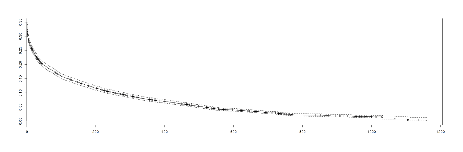
Age of reviewers against probability they will not leave another review
But this is plotting age of reviewers and has no clear connection to calendar time, which was the original hypothesis: that the past 2 years have damaged readership more than the earlier chapters which were posted more timely. In particular, chapter posting seems to have slowed down ~ch62 (published 2010-11-27). So, if we were to look at every user who seems to have begun reading MoR only after that date (as evidenced by their first review postdating ch62’s publication) and compare them to those reading before, do they have additional mortality (above and beyond the low mortality we would expect by being relatively latecomers to MoR, which is adjusted for by the survival curve)? The answer seems to be yes, the survival curves look different when we partition users this way:
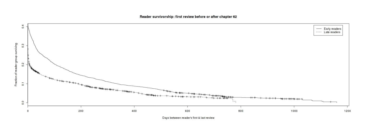
Different mortality curves for 2 groups of reviewers
#   n= 7508, number of events= 6927
#
#            coef exp(coef) se(coef)    z Pr(>|z|)
# LateTRUE 0.2868    1.3322   0.0247 11.6   <2e-16
#
#          exp(coef) exp(-coef) lower .95 upper .95
# LateTRUE      1.33      0.751      1.27       1.4
A pretty clear difference between groups, and an odds ratio of 1.33 (bootstrap 95% CI: 1.22–1.39) is not trivially small. I think we can consider the original hypothesis supported to some degree: the later chapters, either because of the update schedule or perhaps the change in subject matter or attracting a different audience or some other reason, seem to be more likely to lose its readers.
But 2 further minor observations:
Visually, the 2 groups of early & late reviewers look like they might be converging after several years of aging. We might try to interpret this as a ‘hardcore’ vs ‘populist’ distinction: the early reviewers tend to all be early adopters hardcore geeks who become devoted fans in for the long haul, while the late-coming regular people get gradually turned off and only the remaining geeks continue to review.
Can we more specifically nail down this increased mortality to the interval between a reviewer’s last review and the next chapter? So far, no; there is actually a trivially small effect the other direction when we add that as a variable:
#   n= 7326, number of events= 6927
#    (182 observations deleted due to missingness)
#
#               coef exp(coef)  se(coef)     z Pr(>|z|)
# LateTRUE 0.433604 1.542808 0.024906 17.4   <2e-16
# Delay    −0.004236 0.995773 0.000262 −16.2   <2e-16
#
#          exp(coef) exp(-coef) lower .95 upper .95
# LateTRUE     1.543      0.648     1.469     1.620
# Delay        0.996      1.004     0.995     0.996
I interpret this as indicating that an update which is posted after a long drought may be a tiny bit (95% CI: 0.9952–1.9963) more likely to elicit some subsequent reviews (perhaps because extremely long delays are associated with posting multiple chapters quickly), but nevertheless, that overall period with long delays is associated with increased reviewer loss. This makes some post hoc intuitive sense as a polarization effect: if a franchise after a long hiatus finally releases an exciting new work, you may be more likely to discuss or review it, even as the hiatuses make you more likely to finally “check out” for good—you’ll either engage or finally abandon it, but you probably won’t be indifferent.
Source Code
Generation and pre-processing, using the shell & Haskell scripts from before:
data <- read.csv("2013-hpmor-rawreviews.csv", colClasses=c("integer", "Date", "factor"))
users <- unique(data$User)
lifetimes <- data.frame(User=NA, Start=NA, End=NA, FirstChapter=NA, LastChapter=NA)[-1,]
for (i in 1:length(users)) { # isolate a specific user
                  d <- data[data$User == users[i],]
                  # sort by date
                  d <- d[order(d$Date),]

                  first <- head(d, n=1)
                  last <- tail(d, n=1)
                  # build & store new row (per user)
                  new <- data.frame(User=users[i], Start=first$Date, End=last$Date,
                                    FirstChapter=first$Chapter, LastChapter=last$Chapter)
                  lifetimes <- rbind(lifetimes, new)
}
lifetimes$Days <- lifetimes$End - lifetimes$Start
summary(lifetimes$Days)
#    Min. 1st Qu.  Median    Mean 3rd Qu.    Max.
#     0.0     0.0     0.0    55.2     6.0 1160.0
lifetimes$Dead <- lifetimes$LastChapter <= 82

lifetimes$Late <- lifetimes$Start >= as.Date("10-11-27")

# figure out when each chapter was written by its earliest review
chapterDates <- as.Date(NA)
for (i in 1:max(data$Chapter)) { chapterDates[i] <- min(data[data$Chapter==i,]$Date) }

# how long after chapter X was posted did chapter X+1 come along? (obviously NA/unknown for latest chapter)
intervals <- integer(0)
for (i in 1:length(chapterDates)) { intervals[i] <- chapterDates[i+1] - chapterDates[i] }

# look up for every user the relevant delay after their last review
delay <- integer(0)
for (i in 1:nrow(lifetimes)) { delay[i] <- intervals[lifetimes$LastChapter[i]] }
lifetimes$Delay <- delay
Now that we have a clean set of data with the necessary variables like dates, we can analyze:
lifetimes <- read.csv("https://gwern.net/doc/lesswrong-survey/hpmor/2013-hpmor-reviewers.csv",
                       colClasses=c("factor", "Date", "Date", "integer", "integer",
                                    "integer", "logical", "logical","integer"))

library(survival)

surv <- survfit(Surv(Days, Dead, type="right") ~ 1, data=lifetimes)

png(file="~/wiki/doc/lesswrong-survey/hpmor/gwern-survival-overall.png", width = 3*480, height = 1*480)
plot(surv, ylim=c(0, 0.35))
invisible(dev.off())

cmodel <- coxph(Surv(Days, Dead) ~ Late, data=lifetimes)
print(summary(cmodel))

cat("\nTest for assumption violation to confirm the Cox regression:\n")
print(cox.zph(cmodel))

png(file="~/wiki/doc/lesswrong-survey/hpmor/gwern-survival-earlylate-split.jpg", width = 3*480, height = 1*480)
plot(survfit(Surv(Days, Dead) ~ Late, data=lifetimes),
     lty=c(1,2), ylim=c(0, 0.4), main="Reader survivorship: first review before or after chapter 62",
     ylab="Fraction of reader group surviving", xlab="Days between reader's first & last review")
legend("topright", legend=c("Early readers", "Late readers"), lty=c(1 ,2), inset=0.02)
invisible(dev.off())

print(summary(coxph(Surv(Days, Dead) ~ Late + Delay, data=lifetimes)))

cat("\nBegin bootstrap test of coefficient size...\n")
library(boot)
cat("\nGet a subsample, train Cox on it, extract coefficient estimate;\n")
cat("\nfirst the simplest early/late model, then the more complex:\n")
# TODO: factor out duplication
coxCoefficient1 <- function(gb, indices) {
  g <- gb[indices,] # allows boot to select subsample
  # train new regression model on subsample
  cmodel <- coxph(Surv(Days, Dead) ~ Late, data=g)
  return(coef(cmodel))
}
cox1Bs <- boot(data=lifetimes, statistic=coxCoefficient1, R=20000, parallel="multicore", ncpus=4)
print(boot.ci(cox1Bs, type="perc"))
coxCoefficient2 <- function(gb, indices) {
  g <- gb[indices,] # allows boot to select subsample
  # train new regression model on subsample
  cmodel <- coxph(Surv(Days, Dead) ~ Late + Delay, data=g)
  return(coef(cmodel))
}
cox2Bs <- boot(data=lifetimes, statistic=coxCoefficient2, R=20000, parallel="multicore", ncpus=4)
print(boot.ci(cox2Bs, type="perc", index=1)) # `Late`
print(boot.ci(cox2Bs, type="perc", index=2)) # `Delay`