2013 Lewis meditation results
Multilevel modeling of effect of small group’s meditation on math errors
A small group of Quantified Selfers tested themselves daily on arithmetic and engaged in a month of meditation. I analyze their scores with a multilevel model with per-subject grouping, and find the expect result: a small decrease in arithmetic errors which is not statistically-significant, with practice & time-of-day effects (but not day-of-week or weekend effects). This suggests a longer experiment by twice as many experimenters in order to detect this effect.
Quantified Self hobbyist Peter Lewis in April 201313ya began a self-experiment with 11 other hobbyists (with the results posted on Seth Robert’s blog): they used a cellphone app “Math Workout” to do timed simple arithmetic problems (eg. “3.7 + 7.3, 93 + 18, 14 * 7, and 122 + √9”) in an ABA experimental design, where B was practicing mindfulness meditation. This was motivated in part by the observation that, while there is a ton of scientific research on meditation, the studies are often of doubtful quality (he cited a remarkable 2007 collection of meditation meta-analyses).
Lewis thought the results were positive inasmuch as his timings & error rate fell during the meditation period and the falls seemed visually clear when graphed, but some of the participants dropped out and others had graphs that were not so positive.
The interpretation of the data from a statistical point of view was not terribly clear. Lewis & Roberts did not do the analysis. Reading the post, I thought that it was a perfect dataset to try out multilevel models on, as this sort of psychology setup (multiple groups of data per subject, and multiple subjects) is a standard use-case.
Data
The original data was provided by Lewis in an Excel spreadsheet, but formatted in a way I couldn’t make use of. I extracted the data, turned it into a ‘long’ row-by-row format, added IDs for each subject, transformed the dates into R format, and added a variable for each score whether it was on a meditation day. The result was a CSV:
mdtt <- read.csv("https://gwern.net/doc/nootropic/quantified-self/2013-peterlewis-meditation.csv",
                    colClasses=c("factor","Date","character","integer","numeric","logical"))
#     Subject         Date             TimeOfDay           ErrorCount     TestDuration
#  00     :173   Min.   :2013-04-11   Length:886         Min.   : 0.00   Min.   :  61.2
#  03     :126   1st Qu.:2013-04-16   Class :character   1st Qu.: 1.00   1st Qu.:  95.3
#  01     :107   Median :2013-04-21   Mode  :character   Median : 2.00   Median : 119.1
#  04     :106   Mean   :2013-04-21                      Mean   : 3.04   Mean   : 126.1
#  06     : 99   3rd Qu.:2013-04-27                      3rd Qu.: 4.00   3rd Qu.: 143.0
#  05     : 95   Max.   :2013-05-05                      Max.   :25.00   Max.   :2185.7
#  (Other):180                                           NA's   :68      NA's   :69
#  Meditated
#  Mode :logical
#  FALSE:502
#  TRUE :316
#  NA's :68
mdtt <- mdtt[!is.na(mdtt$Subject),]
mdtt <- mdtt[mdtt$TestDuration<400,]
mdtt$ErrorCount <- ifelse(mdtt$ErrorCount<16, mdtt$ErrorCount, c(16))
The TestDuration variable jumps out as bizarre: it goes from 143 seconds to 2185.7 seconds? A closer look shows that the last two entries are 368.42, and then 2185.66. This is a bizarre outlier, so I deleted it. The errors also jump 4 → 25, and a closer look shows a similar jump from 16 to the maximum value 25, which will distort plots later on, so I chose to make 16 the ceiling. We also don’t want the dummy rows which indicate a meditation session, they’re redundant once the Meditated variable has been created. Now that the data is cleaned up and coded, we can look at it. For example, all error scores colored by subject:
Analysis
Descriptive
We have two response variables, number of errors & how long it took to finish the set of 50 arithmetic problems:

library(ggplot2); qplot(Date, jitter(ErrorCount, factor=1.5), color=Subject, data=mdtt, ylab="Number of errors out of 50 problems")
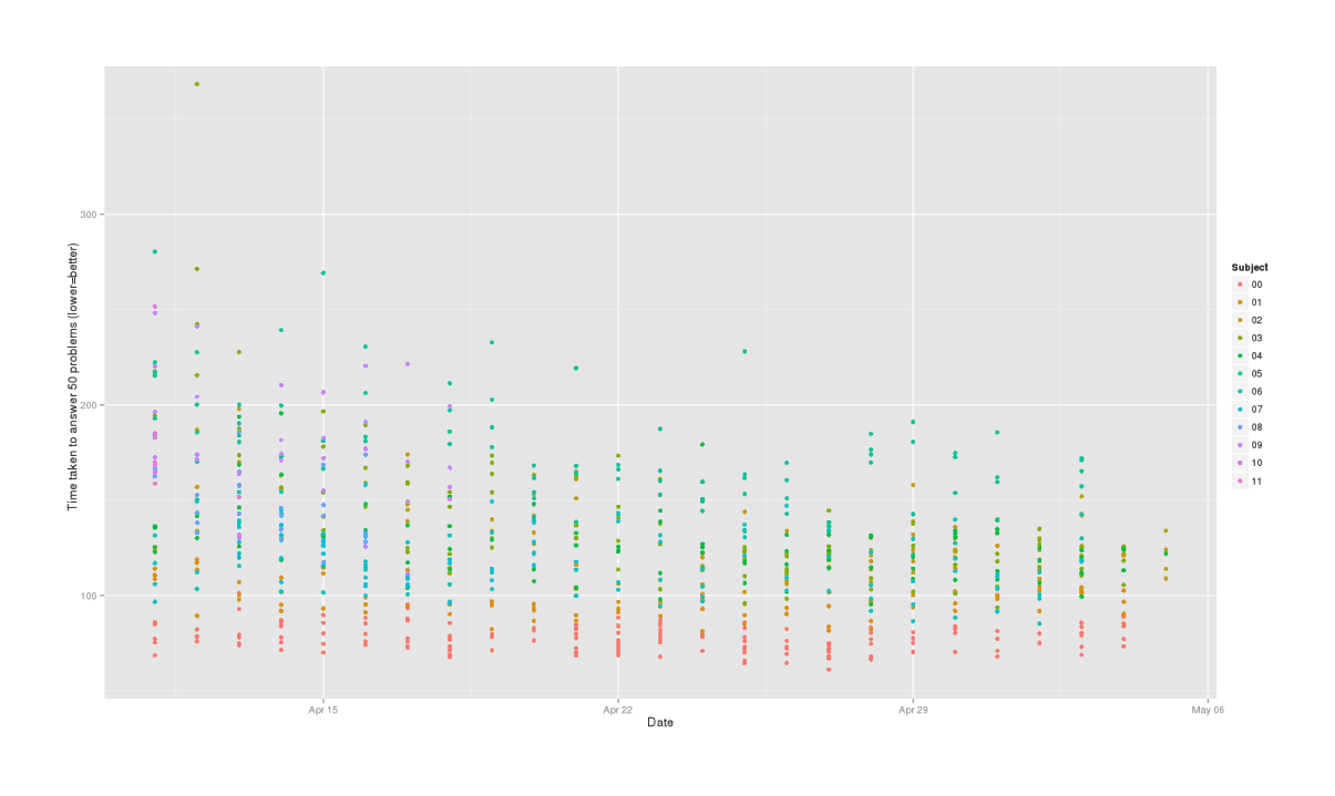
qplot(Date, TestDuration, color=Subject, data=mdtt, ylab="Time taken to answer 50 problems (lower=better)")
We can clearly see a practice effect in both test duration & number of errors, where subjects are gradually getting better over time. We will need to remember to control for that.
Splitting by subject instead and looking at small multiples for any ABA patterns (we delete 3 of the attrited subjects to free up vertical space):
mdtt2 <- mdtt[as.integer(mdtt$Subject) < 9,]
qplot(Date, ErrorCount, color=Meditated, facets=Subject~., data=mdtt2)
qplot(Date, TestDuration, color=Meditated, facets=Subject~., data=mdtt2)
Errors in each phase of ABA, stratified by subject
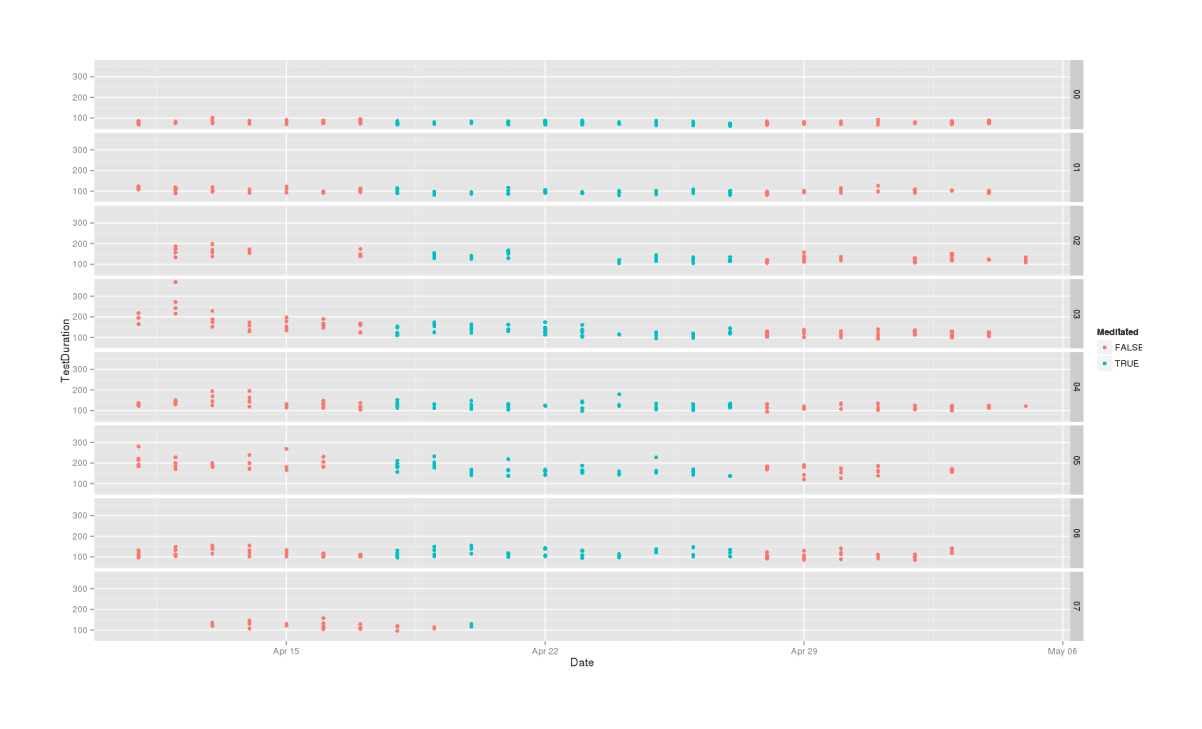
Test time required in each phase, by subject
Overall, these are looking equivocal. There might be something going on, there might not be - ErrorCount looks better than TestDuration, but in both cases, the clear practice effect makes comparison hard.
Goals
Roberts comments:
Another way to improve this experiment would be to do statistical tests that generate p values; this would give a better indication of the strength of the evidence. Because this experiment didn’t reach steady states, the best tests are complicated (eg. comparison of slopes of fitted lines). With steady-state data, these tests are simple (eg. comparison of means).
If you are sophisticated at statistics, you could look for a time-of-day effect (are tests later in the day faster?), a day-of-week effect, and so on. If these effects exist, their removal would make the experiment more sensitive. In my brain-function experiments, I use a small number of problems so that I can adjust for problem difficulty. That isn’t possible here.
p-values are standard in psychology, of course, despite their conceptual & practical problems which help contribute to systematic problems in science, so we’ll calculate one.
But we know in advance what the result will be: greater than 0.05, or non-statistically-significant. A p-value is mostly a function of how much data you have and how large the effect size is - we know a priori that this is a small experiment, and we also know that the effect of meditation on arithmetic scores cannot be huge because otherwise we would have heard of the groundbreaking research & society would make kids meditate before standardized exams & the subjects didn’t do much meditation & they were inexperienced etc. A small experiment on a small effect is guaranteed to not turn in a statistically-significant result, even when there genuinely is an effect, because the experiment doesn’t have much statistical power. In fact, a decrease in errors large enough to reach a statistical-significance of p < 0.05 would be so bizarre & unexpected that it would be grounds for throwing out the data entirely, as someone must be lying or have screwed something up or something have gone terribly wrong somewhere.
So the best we can hope for is to show that there was a benefit at all, rather than a penalty - it’s not clear, visually, that we’ll see better scores once we take into account a practice effect of time. Having shown this, then we can ask additional questions like, “how large an experiment would we need to reach statistical-significance, anyway?”
Multilevel Models
So, we’ll set up a few models in lme4 and compare them. The first model is the simplest: each subject has a different level of base accuracy (intercept), but are influenced the same way by meditation (meditation is a fixed effect):
library(lme4)
mlm1 <- lmer(ErrorCount ~ Meditated + (1|Subject), data=mdtt); mlm1

# ...AIC  BIC logLik deviance REMLdev
#  3793 3812  -1893     3784    3785
# Random effects:
#  Groups   Name        Variance Std.Dev.
#  Subject  (Intercept) 1.37     1.17
#  Residual             5.77     2.40
# Number of obs: 818, groups: Subject, 12
#
# Fixed effects:
#               Estimate Std. Error t value
# (Intercept)      2.892      0.368    7.87
# MeditatedTRUE   -0.213      0.179   -1.19
#
# Correlation of Fixed Effects:
#             (Intr)
# MedittdTRUE -0.139
(This is with a normal distribution family; using a Poisson distribution with family=poisson would give a more accurate model but I am not yet comfortable using or interpreting Poissons.) We get a fixed effect of -0.2 or 1/5 of an error less on meditation days. Not a big effect. The next step is to imagine that besides having differing natural levels of accuracy, meditation may affect some subjects more or less:
mlm2 <- lmer(ErrorCount ~ Meditated + (1+Meditated|Subject), data=mdtt); mlm2

# ...AIC  BIC logLik deviance REMLdev
#  3794 3822  -1891     3780    3782
# Random effects:
#  Groups   Name          Variance Std.Dev. Corr
#  Subject  (Intercept)   1.6378   1.280
#           MeditatedTRUE 0.0913   0.302    -1.000
#  Residual               5.7472   2.397
# Number of obs: 818, groups: Subject, 12
#
# Fixed effects:
#               Estimate Std. Error t value
# (Intercept)      2.881      0.398    7.23
# MeditatedTRUE   -0.144      0.196   -0.74
#
# Correlation of Fixed Effects:
#             (Intr)
# MedittdTRUE -0.568
In this view of things, there’s a weaker effect of meditation: 1/7th of an error less (rather than 1/5th).
But of course, what about the practice effect? The date should matter! Let’s re-run those two models with the date:
mlm1.2 <- lmer(ErrorCount ~ Meditated + Date + (1|Subject), data=mdtt); mlm1.2

# ...  AIC  BIC logLik deviance REMLdev
#  3791 3814  -1890     3772    3781
# Random effects:
#  Groups   Name        Variance Std.Dev.
#  Subject  (Intercept) 1.58     1.26
#  Residual             5.69     2.39
# Number of obs: 818, groups: Subject, 12
#
# Fixed effects:
#               Estimate Std. Error t value
# (Intercept)   698.5757   203.2720    3.44
# MeditatedTRUE  -0.1978     0.1777   -1.11
# Date           -0.0440     0.0129   -3.42
# ...

mlm2.2 <- lmer(ErrorCount ~ Meditated + Date + (1+Meditated|Subject), data=mdtt); mlm2.2
# ...
#   AIC  BIC logLik deviance REMLdev
#  3791 3824  -1889     3769    3777
# Random effects:
#  Groups   Name          Variance Std.Dev. Corr
#  Subject  (Intercept)   1.867    1.37
#           MeditatedTRUE 0.109    0.33     -1.000
#  Residual               5.662    2.38
# Number of obs: 818, groups: Subject, 12
#
# Fixed effects:
#               Estimate Std. Error t value
# (Intercept)   706.2475   203.3645    3.47
# MeditatedTRUE  -0.0928     0.1987   -0.47
# Date           -0.0445     0.0129   -3.46
# ...

## what do the per-subject meditation estimates look like?
## this is similar to what we would see if we did separate regressions on each subject:
ranef(mlm2.2)
# $Subject
#    (Intercept) MeditatedTRUE
# 00    -0.50140       0.11975
# 01    -1.32272       0.31590
# 02    -0.12651       0.03021
# 03     2.99856      -0.71614
# 04     0.96203      -0.22976
# 05     1.33934      -0.31987
# 06    -0.09078       0.02168
# 07     0.04431      -0.01058
# 08    -0.69278       0.16546
# 09    -0.64673       0.15446
# 10    -0.12256       0.02927
# 11    -1.84076       0.43963

## 4/11 have negative meditation estimates
Both agree that there is definitely a practice effect, it’s probably statistically-significant with such large t-values, and the effect size is cumulatively large - at -0.045 errors per day, we’d expect our error rate to decrease by 1.4 errors a month - which is a lot when we remember that the total average errors per session was 3.1!
Time of Day
So, that’s the practice effect verified. What else? Roberts suggested “time-of-day effect (are tests later in the day faster?)” and “day-of-week effect”. First we’ll convert the times to hours and regress on that:
rm(x)
for (i in 1:nrow(mdtt)) { y <- strsplit(mdtt$TimeOfDay[i], ":")[[1]];
                          x[i] <- as.integer(y[[1]])*60 + as.integer(y[[2]]); }
mdtt$Hours <- (x/60)

mlm3 <- lmer(ErrorCount ~ Meditated + Date + Hours + (1|Subject), data=mdtt); mlm3
# ...AIC  BIC logLik deviance REMLdev
#  3789 3817  -1888     3762    3777
# Random effects:
#  Groups   Name        Variance Std.Dev.
#  Subject  (Intercept) 1.52     1.23
#  Residual             5.63     2.37
# Number of obs: 818, groups: Subject, 12
#
# Fixed effects:
#               Estimate Std. Error t value
# (Intercept)   690.4037   202.0927    3.42
# MeditatedTRUE  -0.1875     0.1767   -1.06
# Date           -0.0434     0.0128   -3.40
# Hours          -0.0526     0.0162   -3.25
To my surprise, there really is a time-of-day effect. (I expected that there wouldn’t be enough data to see one, or that it would be a complex squiggle corresponding to circadian rhythms.) And it’s a simple linear one, too, which jumps out when one plots errors against hour:

qplot(Hours, ErrorCount, color=Meditated, data=mdtt)
The lesson here is that doing arithmetic at 7AM is not a good idea. (Would that American high schools could realize this…) But moving on: I really don’t think there’s enough data to get a day-of-week effect as Roberts suggests, so I’ll also do a simpler split on weekends.
mdtt$Day <- weekdays.Date(mdtt$Date)
mdtt$WeekEnd <- mdtt$Day=="Sunday" | mdtt$Day=="Saturday"

mlm4 <- lmer(ErrorCount ~ Meditated + Date + Hours + Day + (1|Subject), data=mdtt); mlm4
# ...AIC  BIC logLik deviance REMLdev
#  3801 3858  -1889     3757    3777
# Random effects:
#  Groups   Name        Variance Std.Dev.
#  Subject  (Intercept) 1.47     1.21
#  Residual             5.64     2.37
# Number of obs: 818, groups: Subject, 12
#
# Fixed effects:
#               Estimate Std. Error t value
# (Intercept)   715.0345   204.1072    3.50
# MeditatedTRUE  -0.1610     0.1803   -0.89
# Date           -0.0450     0.0129   -3.48
# Hours          -0.0518     0.0163   -3.17
# DayMonday      -0.4196     0.3138   -1.34
# DaySaturday    -0.3912     0.2959   -1.32
# DaySunday      -0.1379     0.3032   -0.45
# DayThursday    -0.4688     0.2894   -1.62
# DayTuesday     -0.3116     0.3164   -0.99
# DayWednesday   -0.1052     0.3267   -0.32
# ...
# mlm5 <- lmer(ErrorCount ~ Meditated + Date + Hours + WeekEnd + (1|Subject), data=mdtt); mlm5
# ...
#   AIC  BIC logLik deviance REMLdev
#  3792 3825  -1889     3762    3778
# Random effects:
#  Groups   Name        Variance Std.Dev.
#  Subject  (Intercept) 1.52     1.23
#  Residual             5.63     2.37
# Number of obs: 818, groups: Subject, 12
#
# Fixed effects:
#                Estimate Std. Error t value
# (Intercept)   690.57787  202.44963    3.41
# MeditatedTRUE  -0.18743    0.17684   -1.06
# Date           -0.04345    0.01280   -3.39
# Hours          -0.05263    0.01623   -3.24
# WeekEndTRUE    -0.00412    0.18231   -0.02
# ...
Neither one is impressive. The model using weekends is completely useless, while the model using days looks like it’s overfitting the data.
Which of the 5 models is better, overall and keeping in mind that simplicity is good (we don’t want to overfit the data by throwing in a huge number of random variables which might “explain” variation in error-scores)?
anova(mlm1, mlm2, mlm1.2, mlm2.2, mlm3, mlm4, mlm5)
# ...
#        Df  AIC  BIC logLik Chisq Chi Df Pr(>Chisq)
# mlm1    4 3792 3810  -1892
# mlm1.2  5 3782 3806  -1886 11.44      1    0.00072
# mlm2    6 3792 3821  -1890  0.00      1    1.00000
# mlm3    6 3774 3802  -1881 18.75      0    < 2e-16
# mlm2.2  7 3774 3807  -1880  1.68      1    0.19554
# mlm5    7 3776 3809  -1881  0.00      0    1.00000
# mlm4   12 3781 3838  -1879  4.26      5    0.51227
As we might have guessed, model 3 (Meditated + Date + Hours + (1|Subject)) wins because the practice effect & time-of-day effect matter but apparently not day-of-week in the small dataset we have. (In a larger dataset, then the fancier models might do better.)
Significance
So, in mlm3 the meditation coefficient was -0.1875151ya. How reliable is this meditation coefficient? We’d like a p-value, and the t-values aren’t clear: -1.106?
library(languageR)
mcmc <- pvals.fnc(mlm3)

mcmc$fixed
#               Estimate MCMCmean HPD95lower HPD95upper  pMCMC Pr(>|t|)
# (Intercept)   690.4037 679.5600   268.8057  1069.9631 0.0018   0.0007
# MeditatedTRUE  -0.1875  -0.1837    -0.5400     0.1511 0.2948   0.2889
# Date           -0.0434  -0.0427    -0.0679    -0.0172 0.0018   0.0007
# Hours          -0.0526  -0.0529    -0.0839    -0.0205 0.0012   0.0012
The practice & time-of-day effects are pretty statistically-significant, but we get a p-value of 0.29 for meditation at -0.15 (-0.54-0.15). To put this in perspective: the dataset just isn’t a whole lot of data and the data is heavily loaded on non-meditation data - not such an issue for the date or time-of-day effects which get spread around and estimated evenly, but bad for the meditation data. Another check is by bootstrapping our model from the data and seeing how the meditation estimate varies - does it vary like it did above?
library(boot)
meditationEstimate <- function(dt, indices) {
  d <- dt[indices,] # allows boot to select subsample
  mlm3 <- lmer(ErrorCount ~ Meditated + Date + Hours + (1|Subject), data=d)
  return(fixef(mlm3)[2])
  }
bs <- boot(data=mdtt, statistic=meditationEstimate, R=200000, parallel="multicore", ncpus=4); bs
# ...
# Bootstrap Statistics :
#     original    bias    std. error
# t1*  -0.1656 -0.002162      0.1741

boot.ci(bs)
# ...
# Intervals :
# Level     Percentile
# 95%   (-0.5108,  0.1735 )
# Calculations and Intervals on Original Scale
Very similar: -0.16 (-0.51-0.17).
Power for a Followup Study?
Lewis viewed the collected data as a proto-study, and wants to do a followup experiment which will be better. Besides the obvious methodological improvements one could make like explicitly randomizing blocks of weeks & using better controls (some other mental activity or alternate form of meditation like yoga), how big should the experiment be so that a meditation effect could reach a p < 0.05?
Taking the final effect estimate from my analysis of Lewis’s proto-study at face-value and assume it’s the true effect; how many comparisons of meditation/no-meditation would we have to make to have an 80% chance of detecting the true effect which could pass the 0.05 threshold if we ignored the possibility meditation worsened scores? Roughly estimating it, quite a few. A simple power calculation for the estimated effect of -0.187:
power.t.test(delta = 0.187, sd = 2.682, alternative="one.sided", power=0.8)
# ...
#               n = 2544
#           delta = 0.187
#              sd = 2.682
#       sig.level = 0.05
#           power = 0.8
#     alternative = one.sided
#
# NOTE: n is number in *each* group
(A t-test calculation because I am not yet sure how to do power analysis for a MLM, and this at least will get us in the neighborhood.)
Conclusion
If I’m interpreting the power right, this is not as bad as it looks since each of those n is one math-game, but still. If you have 10 participants and each does 4 games a day, then you’ll need each of your 10 participants to spend 64 days playing the game without meditation (2544 / (10*4) = 64) and another 50 days playing with the meditation. If you could get 20 participants then it’s a more reasonable 2 months total each.
But getting that many fully-compliant volunteers would be quite difficult, and one has to ask: why does one care? It’s not clear that this effect is worth caring about for several reasons:
the value of meditation is over-determined by all the existing research, which in aggregate covers probably hundreds of thousands of subjects. 10 or 30 QSers’ data should not, for a rational person, override or noticeably affect one’s beliefs about the value or meditation. If the existing research says meditation is worthwhile, that is far more trustworthy than this; if it says meditation is not worthwhile, likewise.
the methodology here means that the small effect is not a causal effect of meditation alone, but an unknown melange of countless factors.
What the small decrease means or is caused by, I am agnostic about. I know a lot of people get annoyed when someone brings up methodological issues like expectancy or placebo effects, but with my own blinded self-experiments with nootropics I have felt first-hand placebo effects, and I have been deeply impressed by the results of my dual n-back meta-analysis where simply switching from a passive to an active control group changes the IQ gain from 9.3 IQ points to 2.5.
For me, things like that are the reality behind most self-experiments, and certainly ones with self-selected participants in an unrandomized unblinded experiment with attrition leading to a small effect easily explicable by simply trying a little bit harder.
the metric of arithmetic scores has no clear relation to anything of importance
No one actually cares about simple arithmetic scores. Many results in brain training studies follow a pattern where the training successfully increases scores on some psychological task like digit span, but when researchers look for “far transfer” to things like school grades, no effect can be found. Even if all the other issues could be dealt with and mindfulness meditation did improve arithmetic, what is it a valid proxy for?